statistics – Page 3 – mathstoshare

MCMC for hypothesis testing

A Monte Carlo significance test of the null hypothesis \(X_0 \sim H\) requires creating independent samples \(X_1,\ldots,X_B \sim H\). The idea is if \(X_0 \sim H\) and independently \(X_1,\ldots,X_B\) are i.i.d. from \(H\), then for any test statistic \(T\), the rank of \(T(X_0)\) among \(T(X_0), T(X_1),\ldots, T(X_B)\) is uniformly distributed on \(\{1,\ldots, B+1\}\). This means that if \(T(X_0)\) is one of the \(k\) largest values of \(T(X_b)\), then we can reject the hypothesis \(X \sim H\) at the significance level \(k/(B+1)\).

The advantage of Monte Carlo significance tests is that we do not need an analytic expression for the distribution of \(T(X_0)\) under \(X_0 \sim H\). By generating the i.i.d. samples \(X_1,\ldots,X_B\), we are making an empirical distribution that approximates the theoretical distribution. However, sometimes sampling \(X_1,\ldots, X_B\) is just as intractable as theoretically studying the distribution of \(T(X_0)\) . Often approximate samples based on Markov chain Monte Carlo (MCMC) are used instead. However, these samples are not independent and may not be sampling from the true distribution. This means that a test using MCMC may not be statistically valid

In the 1989 paper Generalized Monte Carlo significance tests, Besag and Clifford propose two methods that solve this exact problem. Their two methods can be used in the same settings where MCMC is used but they are statistically valid and correctly control the Type 1 error. In this post, I will describe just one of the methods – the serial test.

Background on Markov chains

To describe the serial test we will need to introduce some notation. Let \(P\) denote a transition matrix for a Markov chain on a discrete state space \(\mathcal{X}.\) A Markov chain with transition matrix \(P\) thus satisfies,

\(\mathbb{P}(X_n = x_n \mid X_0 = x_0,\ldots, X_{n-1} = x_{n-1}) = P(x_{n-1}, x_n)\)

Suppose that the transition matrix \(P\) has a stationary distribution \(\pi\). This means that if \((X_0, X_1,\ldots)\) is a Markov chain with transition matrix \(P\) and \(X_0\) is distributed according to \(\pi\), then \(X_1\) is also distributed according to \(\pi\). This implies that all \(X_i\) are distributed according to \(\pi\).

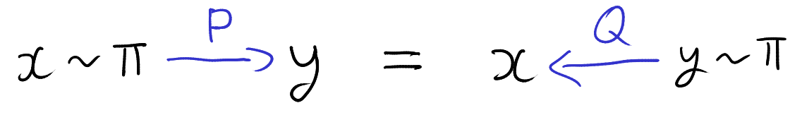
We can construct a new transition matrix \(Q\) from \(P\) and \(\pi\) by \(Q(y,x) = P(x,y) \frac{\pi(x)}{\pi(y)}\). The transition matrix \(Q\) is called the reversal of \(P\). This is because for all \(x\) and \(y\) in \(\mathcal{X}\), \(\pi(x)P(x,y) = \pi(y)Q(x,y)\). That is the chance of drawing \(x\) from \(\pi\) and then transitioning to \(y\) according to \(P\) is equal to the chance of drawing \(y\) from \(\pi\) and then transitioning to \(x\) according to \(Q\)

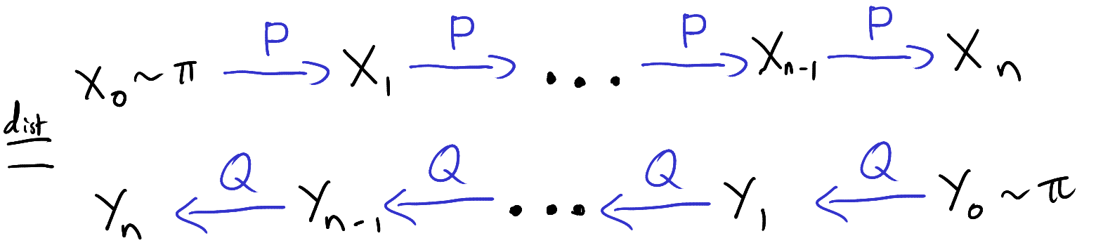
The new transition matrix \(Q\) also allows us to reverse longer runs of the Markov chain. Fix \(n \ge 0\) and let \((X_0,X_1,\ldots,X_n)\) be a Markov chain with transition matrix \(P\) and initial distribution \(\pi\). Also let \((Y_0,Y_1,\ldots,Y_n)\) be a Markov chain with transition matrix \(Q\) and initial distribution \(\pi\), then

\((X_0,X_1,\ldots,X_{n-1}, X_n) \stackrel{dist}{=} (Y_n,Y_{n-1},\ldots, Y_1,Y_0) \),

where \(\stackrel{dist}{=}\) means equal in distribution.

The serial test

Suppose we want to test the hypothesis \(x \sim \pi\) where \(x \in \mathcal{X}\) is our observed data and \(\pi\) is some distribution on \(\mathcal{X}\). To conduct the serial test, we need to construct a Markov chain \(P\) for which \(\pi\) is a stationary distribution. We then also need to construct the reversal \(Q\) described above. There are many possible ways to construct \(P\) such as the Metropolis-Hastings algorithm.

We also need a test statistic \(T\). This is a function \(T:\mathcal{X} \to \mathbb{R}\) which we will use to detect outliers. This function is the same function we would use in a regular Monte Carlo test. Namely, we want to reject the null hypothesis when \(T(x)\) is much larger than we would expect under \(x \sim \pi\).

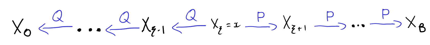
The serial test then proceeds as follows. First we pick \(\xi\) uniformly in \(\{0,1,\ldots,B\}\) and set \(X_\xi = x\). We then generate \((X_\xi, X_{\xi+1},\ldots,X_B)\) as a Markov chain with transition matrix \(P\) that starts at \(X_\xi = x\). Likewise we generate \((X_\xi, X_{\xi-1},\ldots, X_0)\) as a Markov chain that starts from \(Q\).

We then apply \(T\) to each of \((X_0,X_1,\ldots,X_\xi,\ldots,X_B)\) and count the number of \(b \in \{0,1,\ldots,B\}\) such that \(T(X_b) \ge T(X_\xi) = T(x)\). If there are \(k\) such \(b\), then the reported p-value of our test is \(k/(B+1)\).

We will now show that this test produces a valid p-value. That is, when \(x \sim \pi\), the probability that \(k/(B+1)\) is less than \(\alpha\) is at most \(\alpha\). In symbols,

\(\mathbb{P}\left( \frac{\#\{b: T(X_b) \ge T(X_\xi)\}}{B+1} \le \alpha \right) \le \alpha\)

Under the null hypothesis \(x \sim \pi\), \((X_\xi, X_{\xi-1},\ldots, X_0)\) is equal in distribution to generating \(X_0\) from \(\pi\) and using the transition matrix \(P\) to go from \(X_i\) to \(X_{i+1}\).

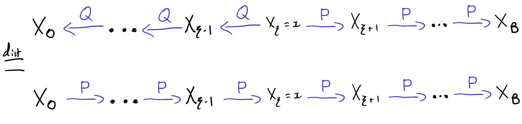
Thus, under the null hypothesis, the distribution of \((X_0,X_1,\ldots,X_B)\) does not depend on \(\xi\). The entire procedure is equivalent to generating a Markov chain \(\mathbf{X} = (X_0,X_1,\ldots,X_B)\) with initial distribution \(\pi\) and transition matrix \(P\), and then choosing \(\xi \in \{0,1,\ldots,B\}\) independently of \(\mathbf{X}\). This is enough to show that the serial method produces valid p-values. The idea is that since the distribution of \(\mathbf{X}\) does not depend on \(\xi\) and \(\xi\) is uniformly distributed on \(\{0,1,\ldots,B\}\), the probability that \(T(X_\xi)\) is in the top \(\alpha\) proportion of \(T(X_b)\) should be at most \(\alpha\). This is proved more formally below.

For each \(i \in \{0,1,\ldots,B\}\), let \(A_i\) be the event that \(T(X_i)\) is in the top \(\alpha\) proportion of \(T(X_0),\ldots,T(X_B)\). That is,

\(A_i = \left\{ \frac{\# \{b : T(X_b) \ge T(X_i)\} }{B+1} \le \alpha \right\}\).

Let \(I_{A_i}\) be the indicator function for the event \(A_i\). Since at must \(\alpha(B+1)\) values of \(i\) can be in the top \(\alpha\) fraction of \(T(X_0),\ldots,T(X_B)\), we have that

\(\sum_{i=0}^B I_{A_i} \le \alpha(B+1)\),

Therefor, by linearity of expectations,

\(\sum_{i=0}^B \mathbb{P}(A_i) \le \alpha(B+1)\)

By the law of total probability we have that \(\mathbb{P}\left(\frac{\#\{b: T(X_b) \ge T(X_\xi)\}}{B+1} \le \alpha \right)\) is equal to

\(\sum_{i=0}^B \mathbb{P}\left(\frac{\#\{b: T(X_b) \ge T(X_\xi)\}}{B+1} \le \alpha | \xi = i\right)\mathbb{P}(\xi = i)\),

Since \(\xi\) is uniform on \(\{0,\ldots,B\}\), \(\mathbb{P}(\xi = i)\) is \(\frac{1}{B+1}\) for all \(i\). Furthermore, by independence of \(\xi\) and \(\mathbf{X}\), we have

\(\mathbb{P}\left(\frac{\#\{b: T(X_b) \ge T(X_\xi)\}}{B+1} \le \alpha | \xi = i\right) = \mathbb{P}(A_i)\).

Thus, by our previous bound,

\(\mathbb{P}\left(\frac{\#\{b: T(X_b) \ge T(X_\xi)\}}{B+1} \le \alpha \right) = \frac{1}{B+1}\sum_{i=0}^B \mathbb{P}(A_i) \le \alpha\).

Applications

In the original paper by Besag and Clifford, the authors discuss how this procedure can be used to perform goodness-of-fit tests. They construct Markov chains that can test the Rasch model or the Ising model. More broadly the method can be used to tests goodness-of-fit tests for any exponential family by using the Markov chains developed by Diaconis and Sturmfels.

A similar method has also been applied more recently to detect Gerrymandering. In this setting, the null hypothesis is the uniform distribution on all valid redistrictings of a state and the test statistics \(T\) measure the political advantage of a given districting.

References

How to Bake Pi, Sherman-Morrison and log-sum-exp

A few months ago, I had the pleasure of reading Eugenia Cheng‘s book How to Bake Pi. Each chapter starts with a recipe which Cheng links to the mathematical concepts contained in the chapter. The book is full of interesting connections between mathematics and the rest of the world.

One of my favourite ideas in the book is something Cheng writes about equations and the humble equals sign: \(=\). She explains that when an equation says two things are equal we very rarely mean that they are exactly the same thing. What we really mean is that the two things are the same in some ways even though they may be different in others.

One example that Cheng gives is the equation \(a + b = b+a\). This is such a familiar statement that you might really think that \(a+b\) and \(b+a\) are the same thing. Indeed, if \(a\) and \(b\) are any numbers, then the number you get when you calculate \(a + b\) is the same as the number you get when you calculate \(b + a\). But calculating \(a+b\) could be very different from calculating \(b+a\). A young child might calculate \(a+b\) by starting with \(a\) and then counting one-by-one from \(a\) to \(a + b\). If \(a\) is \(1\) and \(b\) is \(20\), then calculating \(a + b\) requires counting from \(1\) to \(21\) but calculating \(b+a\) simply amounts to counting from \(20\) to \(21\). The first process takes way longer than the second and the child might disagree that \(1 + 20\) is the same as \(20 + 1\).

In How to Bake Pi, Cheng explains that a crucial idea behind equality is context. When someone says that two things are equal we really mean that they are equal in the context we care about. Cheng talks about how context is crucial through-out mathematics and introduces a little bit of category theory as a tool for moving between different contexts. I think that this idea of context is really illuminating and I wanted to share some examples where “\(=\)” doesn’t mean “exactly the same as”.

The Sherman-Morrison formula

The Sherman-Morrison formula is a result from linear algebra that says for any invertible matrix \(A \in \mathbb{R}^{n\times n}\) and any pair of vectors \(u,v \in \mathbb{R}^n\), if \(v^TA^{-1}u \neq -1\), then \(A + uv^T\) is invertible and

\((A + uv^T)^{-1} = A^{-1} + \frac{A^{-1}uv^TA^{-1}}{1 + v^TA^{-1}u}\)

Here “\(=\)” means the following:

You can take any natural number \(n\), any matrix \(A\) of size \(n\) by \(n\), and any length \(n\)-vectors \(u\) and \(v\) that satisfy the above condition.
If you take all those things and carry out all the matrix multiplications, additions and inversions on the left and all the matrix multiplications, additions and inversions on the right, then you will end up with exactly the same matrix in both cases.

But depending on the context, the equation on one side of “\(=\)” may be much easier than the other. Although the right hand side looks a lot more complicated, it is much easier to compute in one important context. This context is when we have already calculated the matrix \(A^{-1}\) and now want the inverse of \(A + uv^T\). The left hand side naively computes \(A + uv^T\) which takes \(O(n^3)\) computations since we have to invert a \(n \times n\) matrix. On the right hand side, we only need to compute a small number of matrix-vector products and then add two matrices together. This bring the computational cost down to \(O(n^2)\).

These cost saving measures come up a lot when studying linear regression. The Sherman-Morrison formula can be used to update regression coefficients when a new data point is added. Similarly, the Sherman-Morrison formula can be used to quickly calculate the fitted values in leave-one-out cross validation.

log-sum-exp

This second example also has connections to statistics. In a mixture model, we assume that each data point \(Y\) comes from a distribution of the form:

\(p(y|\pi,\theta) = \sum_{k=1}^K \pi_k p(y | \theta_k)\),

where \(\pi \) is a vector and \(\pi_k\) is equal to the probability that \(Y\) came from class \(k\). The parameters \(\theta_k \in\mathbb{R}^p\) are the parameters for the \(k^{th}\) group.The log-likelihood is thus,

\(\log\left(\sum_{k=1}^K \pi_k p(y | \theta_k)\right) = \log\left(\sum_{k=1}^K \exp(\eta_{k})\right)\),

where \(\eta_{k} = \log(\pi_k p(y| \theta_k))\). We can see that the log-likelihood is of the form log-sum-exp. Calculating a log-sum-exp can cause issues with numerical stability. For instance if \(K = 3\) and \(\eta_k = 1000\), for all \(k=1,2,3\), then the final answer is simply \(\log(3)+1000\). However, as soon as we try to calculate \(\exp(1000)\) on a computer, we’ll be in trouble.

The solution is to use the following equality, for any \(\beta \in \mathbb{R}\),

\(\log\left(\sum_{k=1}^K \exp(\eta_k) \right) = \beta + \log\left(\sum_{k=1}^K \exp(\beta – \eta_k)\right)\).

Proving the above identity is a nice exercise in the laws of logarithm’s and exponential’s, but with a clever choice of \(\beta\) we can more safely compute the log-sum-exp expression. For instance, in the documentation for pytorch’s implementation of logsumexp() they take \(\beta\) to be the maximum of \(\eta_k\). This (hopefully) makes each of the terms \(\beta – \eta_k\) a reasonable size and avoids any numerical issues.

Again, the left and right hand sides of the above equation might be the same number, but in the context of having to use computers with limited precision, they represent very different calculations.

Beyond How to Bake Pi

Eugenia Cheng has recently published a new book called The Joy of Abstraction. I’m just over half way through and it’s been a really engaging and interesting introduction to category theory. I’m looking forward to reading the rest of it and getting more insight from Eugenia Cheng’s great mathematical writing.

Looking back on the blog

Next week I’ll be starting the second year of my statistics PhD. I’ve learnt a lot from taking the first year classes and studying for the qualifying exams. Some of what I’ve learnt has given me a new perspective on some of my old blog posts. Here are three things that I’ve written about before and I now understand better.

1. The Pi-Lambda Theorem

An early post on this blog was titled “A minimal counterexample in probability theory“. The post was about a theorem from the probability course offered at the Australian National University. The theorem states that if two probability measures agree on a collection of subsets and the collection is closed under finite intersections, then the two probability measures agree on the \(\sigma\)-algebra generated by the collection. In my post I give an example which shows that you need the collection to be closed under finite intersections. I also show that you need to have at least four points in the space to find such an example.

What I didn’t know then is that the above theorem is really a corollary of Dykin’s \(\pi – \lambda\) theorem. This theorem was proved in my first graduate probability course which was taught by Persi Diaconis. Professor Diaconis kept a running tally of how many times we used the \(\pi – \lambda\) theorem in his course and we got up to at least 10. (For more appearances by Professor Diaconis on this blog see here, here and here).

If I were to write the above post again, I would talk about the \(\pi – \lambda\) theorem and rename the post “The smallest \(\lambda\)-system”. The example given in my post is really about needing at least four points to find a \(\lambda\)-system that is not a \(\sigma\)-algebra.

2. Mallow’s C_p statistic

The very first blog post I wrote was called “Complexity Penalties in Statistical Learning“. I wasn’t sure if I would write a second and so I didn’t set up a WordPress account. I instead put the post on the website LessWrong. I no longer associate myself with the rationality community but posting to LessWrong was straight forward and helped me reach more people.

The post was inspired in two ways by the 2019 AMSI summer school. First, the content is from the statistical learning course I took at the summer school. Second, at the career fair many employers advised us to work on our writing skills. I don’t know if would have started blogging if not for the AMSI Summer School.

I didn’t know it at the time but the blog post is really about Mallow’s C_p statistic. Mallow’s C_p statistic is an estimate of the test error of a regression model fit using ordinary least squares. The Mallow’s C_p is equal to the training error plus a “complexity penalty” which takes into account the number of parameters. In the blog post I talk about model complexity and over-fitting. I also write down and explain Mallow’s C_p in the special case of polynomial regression.

In the summer school course I took, I don’t remember the name Mallow’s C_p being used but I thought it was a great idea and enjoyed writing about it. The next time encountered Mallow’s C_p was in the linear models course I took last fall. I was delighted to see it again and learn how it fit into a bigger picture. More recently, I read Brad Efron’s paper “How Biased is the Apparent Error Rate of a Prediction Rule ?“. The paper introduces the idea of “effective degrees of freedom” and expands on the ideas behind the C_p statistic.

Incidentally, enrolment is now open for the 2023 AMSI Summer School! This summer it will be hosted at the University of Melbourne. I encourage any Australia mathematics or statistics students reading this to take a look and apply. I really enjoyed going in both 2019 and 2020. (Also if you click on the above link you can try to spot me in the group photo of everyone wearing read shirts!)

3. Finitely additive probability measures

In “Finitely additive measures” I talk about how hard it is to define a finitely additive measure on the set of natural numbers that is not countably additive. In particular, I talked about needing to use the Hahn — Banach extension theorem to extend the natural density from the collection of sets with density to the collection of all subsets of the natural numbers.

There were a number of homework problems in my first graduate probability course that relate to this post. We proved that the sets with density are not closed under finite unions and we showed that the square free numbers have density \(6/\pi^2\).

We also proved that any finite measure defined on an algebra of subsets can be extend to the collection of all subsets. This proof used Zorn’s lemma and the resulting measure is far from unique. The use of Zorn’s lemma relates to the main idea in my blog, that defining an additive probability measure is in some sense non-constructive.

Sampling from the non-central chi-squared distribution

The non-central chi-squared distribution is a generalisation of the regular chi-squared distribution. The chi-squared distribution turns up in many statistical tests as the (approximate) distribution of a test statistic under the null hypothesis. Under alternative hypotheses, those same statistics often have approximate non-central chi-squared distributions.

This means that the non-central chi-squared distribution is often used to study the power of said statistical tests. In this post I give the definition of the non-central chi-squared distribution, discuss an important invariance property and show how to efficiently sample from this distribution.

Definition

Let \(Z\) be a normally distributed random vector with mean \(0\) and covariance \(I_n\). Given a vector \(\mu \in \mathbb{R}^n\), the non-central chi-squared distribution with \(n\) degrees of freedom and non-centrality parameter \(\Vert \mu\Vert_2^2\) is the distribution of the quantity

\(\Vert Z+\mu \Vert_2^2 = \sum\limits_{i=1}^n (Z_i+\mu_i)^2. \)

This distribution is denoted by \(\chi^2_n(\Vert \mu \Vert_2^2)\). As this notation suggests, the distribution of \(\Vert Z+\mu \Vert_2^2\) depends only on \(\Vert \mu \Vert_2^2\), the norm of \(\mu\). The first few times I heard this fact, I had no idea why it would be true (and even found it a little spooky). But, as we will see below, the result is actually a simply consequence of the fact that standard normal vectors are invariant under rotations.

Rotational invariance

Suppose that we have two vectors \(\mu, \nu \in \mathbb{R}^n\) such that \(\Vert \mu\Vert_2^2 = \Vert \nu \Vert_2^2\). We wish to show that if \(Z \sim \mathcal{N}(0,I_n)\), then

\(\Vert Z+\mu \Vert_2^2\) has the same distribution as \(\Vert Z + \nu \Vert_2^2\).

Since \(\mu\) and \(\nu\) have the same norm there exists an orthogonal matrix \(U \in \mathbb{R}^{n \times n}\) such that \(U\mu = \nu\). Since \(U\) is orthogonal and \(Z \sim \mathcal{N}(0,I_n)\), we have \(Z’=UZ \sim \mathcal{N}(U0,UU^T) = \mathcal{N}(0,I_n)\). Furthermore, since \(U\) is orthogonal, \(U\) preserves the norm \(\Vert \cdot \Vert_2^2\). This is because, for all \(x \in \mathbb{R}^n\),

\(\Vert Ux\Vert_2^2 = (Ux)^TUx = x^TU^TUx=x^Tx=\Vert x\Vert_2^2.\)

Putting all these pieces together we have

\(\Vert Z+\mu \Vert_2^2 = \Vert U(Z+\mu)\Vert_2^2 = \Vert UZ + U\mu \Vert_2^2 = \Vert Z’+\nu \Vert_2^2\).

Since \(Z\) and \(Z’\) have the same distribution, we can conclude that \( \Vert Z’+\nu \Vert_2^2\) has the same distribution as \(\Vert Z + \nu \Vert\). Since \(\Vert Z + \mu \Vert_2^2 = \Vert Z’+\nu \Vert_2^2\), we are done.

Sampling

Above we showed that the distribution of the non-central chi-squared distribution, \(\chi^2_n(\Vert \mu\Vert_2^2)\) depends only on the norm of the vector \(\mu\). We will now use this to provide an algorithm that can efficiently generate samples from \(\chi^2_n(\Vert \mu \Vert_2^2)\).

A naive way to sample from \(\chi^2_n(\Vert \mu \Vert_2^2)\) would be to sample \(n\) independent standard normal random variables \(Z_i\) and then return \(\sum_{i=1}^n (Z_i+\mu_i)^2\). But for large values of \(n\) this would be very slow as we have to simulate \(n\) auxiliary random variables \(Z_i\) for each sample from \(\chi^2_n(\Vert \mu \Vert_2^2)\). This approach would not scale well if we needed many samples.

An alternative approach uses the rotation invariance described above. The distribution \(\chi^2_n(\Vert \mu \Vert_2^2)\) depends only on \(\Vert \mu \Vert_2^2\) and not directly on \(\mu\). Thus, given \(\mu\), we could instead work with \(\nu = \Vert \mu \Vert_2 e_1\) where \(e_1\) is the vector with a \(1\) in the first coordinate and \(0\)s in all other coordinates. If we use \(\nu\) instead of \(\mu\), we have

\(\sum\limits_{i=1}^n (Z_i+\nu_i)^2 = (Z_1+\Vert \mu \Vert_2)^2 + \sum\limits_{i=2}^{n}Z_i^2.\)

The sum \(\sum_{i=2}^n Z_i^2\) follows the regular chi-squared distribution with \(n-1\) degrees of freedom and is independent of \(Z_1\). The regular chi-squared distribution is a special case of the gamma distribution and can be effectively sampled with rejection sampling for large shape parameter (see here).

The shape parameter for \(\sum_{i=2}^n Z_i^2\) is \(\frac{n-1}{2}\), so for large values of \(n\) we can efficiently sample a value \(Y\) that follows that same distribution as \(\sum_{i=2}^n Z_i^2 \sim \chi^2_{n-1}\). Finally to get a sample from \(\chi^2_n(\Vert \mu \Vert_2^2)\) we independently sample \(Z_1\), and then return the sum \((Z_1+\Vert \mu\Vert_2)^2 +Y\).

Conclusion

In this post, we saw that the rotational invariance of the standard normal distribution gives a similar invariance for the non-central chi-squared distribution.

This invariance allowed us to efficiently sample from the non-central chi-squared distribution. The sampling procedure worked by reducing the problem to sampling from the regular chi-squared distribution.

The same invariance property is also used to calculate the cumulative distribution function and density of the non-central chi-squared distribution. Although the resulting formulas are not for the faint of heart.

The Singular Value Decomposition (SVD)

The singular value decomposition (SVD) is a powerful matrix decomposition. It is used all the time in statistics and numerical linear algebra. The SVD is at the heart of the principal component analysis, it demonstrates what’s going on in ridge regression and it is one way to construct the Moore-Penrose inverse of a matrix. For more SVD love, see the tweets below.

A tweet by Women in Statistics and Data Science about the SVD.
The full thread is here https://twitter.com/WomenInStat/status/1285610321747611653?s=20&t=Elj62mGSc9gINHvbwt82Zw

In this post I’ll define the SVD and prove that it always exists. At the end we’ll look at some pictures to better understand what’s going on.

Definition

Let \(X\) be a \(n \times p\) matrix. We will define the singular value decomposition first in the case \(n \ge p\). The SVD consists of three matrix \(U \in \mathbb{R}^{n \times p}, \Sigma \in \mathbb{R}^{p \times p}\) and \(V \in \mathbb{R}^{p \times p}\) such that \(X = U\Sigma V^T\). The matrix \(\Sigma\) is required to be diagonal with non-negative diagonal entries \(\sigma_1 \ge \sigma_2 \ge \ldots \ge \sigma_p \ge 0\). These numbers are called the singular values of \(X\). The matrices \(U\) and \(V\) are required to orthogonal matrices so that \(U^TU=V^TV = I_p\), the \(p \times p\) identity matrix. Note that since \(V\) is square we also have \(VV^T=I_p\) however we won’t have \(UU^T = I_n\) unless \(n = p\).

In the case when \(n \le p\), we can define the SVD of \(X\) in terms of the SVD of \(X^T\). Let \(\widetilde{U} \in \mathbb{R}^{p \times n}, \widetilde{\Sigma} \in \mathbb{R}^{n \times n}\) and \(\widetilde{V} \in \mathbb{R}^{n \times n}\) be the SVD of \(X^T\) so that \(X^T=\widetilde{U}\widetilde{\Sigma}\widetilde{V}^T\). The SVD of \(X\) is then given by transposing both sides of this equation giving \(U = \widetilde{V}, \Sigma = \widetilde{\Sigma}^T=\widetilde{\Sigma}\) and \(V = \widetilde{U}\).

Construction

The SVD of a matrix can be found by iteratively solving an optimisation problem. We will first describe an iterative procedure that produces matrices \(U \in \mathbb{R}^{n \times p}, \Sigma \in \mathbb{R}^{p \times p}\) and \(V \in \mathbb{R}^{p \times p}\). We will then verify that \(U,\Sigma \) and \(V\) satisfy the defining properties of the SVD.

We will construct the matrices \(U\) and \(V\) one column at a time and we will construct the diagonal matrix \(\Sigma\) one entry at a time. To construct the first columns and entries, recall that the matrix \(X\) is really a linear function from \(\mathbb{R}^p\) to \(\mathbb{R}^n\) given by \(v \mapsto Xv\). We can thus define the operator norm of \(X\) via

\(\Vert X \Vert = \sup\left\{ \|Xv\|_2 : \|v\|_2 =1\right\},\)

where \(\|v\|_2\) represents the Euclidean norm of \(v \in \mathbb{R}^p\) and \(\|Xv\|_2\) is the Euclidean norm of \(Xv \in \mathbb{R}^n\). The set of vectors \(\{v \in \mathbb{R} : \|v\|_2 = 1 \}\) is a compact set and the function \(v \mapsto \|Xv\|_2\) is continuous. Thus, the supremum used to define \(\Vert X \Vert\) is achieved at some vector \(v_1 \in \mathbb{R}^p\). Define \(\sigma_1 = \|X v_1\|_2\). If \(\sigma_1 \neq 0\), then define \(u_1 = Xv_1/\sigma_1 \in \mathbb{R}^n\). If \(\sigma_1 = 0\), then define \(u_1\) to be an arbitrary vector in \(\mathbb{R}^n\) with \(\|u\|_2 = 1\). To summarise we have

\(v_1 \in \mathbb{R}^p\) with \(\|v_1\|_2 = 1\).
\(\sigma_1 = \|X\| = \|Xv_1\|_2\).
\(u_1 \in \mathbb{R}^n\) with \(\|u_1\|_2=1\) and \(Xv_1 = \sigma_1u_1\).

We have now started to fill in our SVD. The number \(\sigma_1 \ge 0\) is the first singular value of \(X\) and the vectors \(v_1\) and \(u_1\) will be the first columns of the matrices \(V\) and \(U\) respectively.

Now suppose that we have found the first \(k\) singular values \(\sigma_1,\ldots,\sigma_k\) and the first \(k\) columns of \(V\) and \(U\). If \(k = p\), then we are done. Otherwise we repeat a similar process.

Let \(v_1,\ldots,v_k\) and \(u_1,\ldots,u_k\) be the first \(k\) columns of \(V\) and \(U\). The vectors \(v_1,\ldots,v_k\) split \(\mathbb{R}^p\) into two subspaces. These subspaces are \(S_1 = \text{span}\{v_1,\ldots,v_k\}\) and \(S_2 = S_1^\perp\), the orthogonal compliment of \(S_1\). By restricting \(X\) to \(S_2\) we get a new linear map \(X_{|S_2} : S_2 \to \mathbb{R}^n\). Like before, the operator norm of \(X_{|S_2}\) is defined to be

\(\|X_{|S_2}\| = \sup\{\|X_{|S_2}v\|_2:v \in S_2, \|v\|_2=1\}\).

Since \(S_2 = \text{span}\{v_1,\ldots,v_k\}^\perp\) we must have

\(\|X_{|S_2}\| = \sup\{\|Xv\|_2:v \in \mathbb{R}^p, \|v\|_2=1, v_j^Tv = 0 \text{ for } j=1,\ldots,k\}.\)

The set \(\{v \in \mathbb{R}^p : \|v\|_2=1, v_j^Tv=0\text{ for } j=1,\ldots,k\}\) is a compact set and thus there exists a vector \(v_{k+1}\) such that \(\|Xv_{k+1}\|_2 = \|X_{|S_2}\|\). As before define \(\sigma_{k+1} = \|Xv_{k+1}\|_2\) and \(u_{k+1} = Xv_{k+1}/\sigma_{k+1}\) if \(\sigma_{k+1}\neq 0\). If \(\sigma_{k+1} = 0\), then define \(u_{k+1}\) to be any vector in \(\mathbb{R}^{n}\) that is orthogonal to \(u_1,u_2,\ldots,u_k\).

This process repeats until eventually \(k = p\) and we have produced matrices \(U \in \mathbb{R}^{n \times p}, \Sigma \in \mathbb{R}^{p \times p}\) and \(V \in \mathbb{R}^{p \times p}\). In the next section, we will argue that these three matrices satisfy the properties of the SVD.

Correctness

The defining properties of the SVD were given at the start of this post. We will see that most of the properties follow immediately from the construction but one of them requires a bit more analysis. Let \(U = [u_1,\ldots,u_p]\), \(\Sigma = \text{diag}(\sigma_1,\ldots,\sigma_p)\) and \(V= [v_1,\ldots,v_p]\) be the output from the above construction.

First note that by construction \(v_1,\ldots, v_p\) are orthogonal since we always had \(v_{k+1} \in \text{span}\{v_1,\ldots,v_k\}^\perp\). It follows that the matrix \(V\) is orthogonal and so \(V^TV=VV^T=I_p\).

The matrix \(\Sigma\) is diagonal by construction. Furthermore, we have that \(\sigma_{k+1} \le \sigma_k\) for every \(k\). This is because both \(\sigma_k\) and \(\sigma_{k+1}\) were defined as maximum value of \(\|Xv\|_2\) over different subsets of \(\mathbb{R}^p\). The subset for \(\sigma_k\) contained the subset for \(\sigma_{k+1}\) and thus \(\sigma_k \ge \sigma_{k+1}\).

We’ll next verify that \(X = U\Sigma V^T\). Since \(V\) is orthogonal, the vectors \(v_1,\ldots,v_p\) form an orthonormal basis for \(\mathbb{R}^p\). It thus suffices to check that \(Xv_k = U\Sigma V^Tv_k\) for \(k = 1,\ldots,p\). Again by the orthogonality of \(V\) we have that \(V^Tv_k = e_k\), the \(k^{th}\) standard basis vector. Thus,

\(U\Sigma V^Tv_k = U\Sigma e_k = U\sigma_k e_k = \sigma_k u_k.\)

Above, we used that \(\Sigma\) was a diagonal matrix and that \(u_k\) is the \(k^{th}\) column of \(U\). If \(\sigma_k \neq 0\), then \(\sigma_k u_k = Xv_k\) by definition. If \(\sigma_k =0\), then \(\|Xv_k\|_2=0\) and so \(Xv_k = 0 = \sigma_ku_k\) also. Thus, in either case, \(U\Sigma V^Tv_k = Xv_k\) and so \(U\Sigma V^T = X\).

The last property we need to verify is that \(U\) is orthogonal. Note that this isn’t obvious. At each stage of the process, we made sure that \(v_{k+1} \in \text{span}\{v_1,\ldots,v_k\}^\perp\). However, in the case that \(\sigma_{k+1} \neq 0\), we simply defined \(u_{k+1} = Xv_{k+1}/\sigma_{k+1}\). It is not clear why this would imply that \(u_{k+1}\) is orthogonal to \(u_1,\ldots,u_k\).

It turns out that a geometric argument is needed to show this. The idea is that if \(u_{k+1}\) was not orthogonal to \(u_j\) for some \(j \le k\), then \(v_j\) couldn’t have been the value that maximises \(\|Xv\|_2\).

Let \(u_{k}\) and \(u_j\) be two columns of \(U\) with \(j < k\) and \(\sigma_j,\sigma_k > 0\). We wish to show that \(u_j^Tu_k = 0\). To show this we will use the fact that \(v_j\) and \(v_k\) are orthonormal and perform “polar-interpolation“. That is, for \(\lambda \in [0,1]\), define

\(v_\lambda = \sqrt{1-\lambda}\cdot v_{j}-\sqrt{\lambda} \cdot v_k.\)

Since \(v_{j}\) and \(v_k\) are orthogonal, we have that

\(\|v_\lambda\|_2^2 = (1-\lambda)\|v_{j}\|_2^2+\lambda\|v_k\|_2^2 = (1-\lambda)+\lambda = 1.\)

Furthermore \(v_\lambda\) is orthogonal to \(v_1,\ldots,v_{j-1}\). Thus, by definition of \(v_j\),

\(\|Xv_\lambda\|_2^2 \le \sigma_j^2 = \|Xv_j\|_2^2.\)

By the linearity of \(X\) and the definitions of \(u_j,u_k\),

\(\|Xv_\lambda\|_2^2 = \|\sigma_j\sqrt{1-\lambda}\cdot u_j+\sigma_{k+1}\sqrt{\lambda}\cdot u_{k+1}\|_2^2\).

Since \(Xv_j = \sigma_ju_j\) and \(Xv_{k+1}=\sigma_{k+1}u_{k+1}\), we have

\((1-\lambda)\sigma_j^2 + 2\sqrt{\lambda(1-\lambda)}\cdot \sigma_1\sigma_2 u_j^Tu_{k}+\lambda\sigma_k^2 = \|Xv_\lambda\|_2^2 \le \sigma_j^2\)

Rearranging and dividing by \(\sqrt{\lambda}\) gives,

\(2\sqrt{1-\lambda}\cdot \sigma_1\sigma_2 u_j^Tu_k \le \sqrt{\lambda}\cdot(\sigma_j^2-\sigma_k^2).\) for all \(\lambda \in (0,1]\)

Taking \(\lambda \to 0\) gives \(u_j^Tu_k \le 0\). Performing the same polar interpolation with \(v_\lambda’ = \sqrt{1-\lambda}v_j – \sqrt{\lambda}v_k\) shows that \(-u_j^Tu_k \le 0\) and hence \(u_j^Tu_k = 0\).

We have thus proved that \(U\) is orthogonal. This proof is pretty “slick” but it isn’t very illuminating. To better demonstrate the concept, I made an interactive Desmos graph that you can access here.

This graph shows example vectors \(u_j, u_k \in \mathbb{R}^2\). The vector \(u_j\) is fixed at \((1,0)\) and a quarter circle of radius \(1\) is drawn. Any vectors \(u\) that are outside this circle have \(\|u\|_2 > 1 = \|u_j\|_2\).

The vector \(u_k\) can be moved around inside this quarter circle. This can be done either cby licking and dragging on the point or changing that values of \(a\) and \(b\) on the left. The red curve is the path of

\(\lambda \mapsto \sqrt{1-\lambda}\cdot u_j+\sqrt{\lambda}\cdot u_k\).

As \(\lambda\) goes from \(0\) to \(1\), the path travels from \(u_j\) to \(u_k\).

Note that there is a portion of the red curve near \(u_j\) that is outside the black circle. This corresponds to a small value of \(\lambda > 0\) that results in \(\|X v_\lambda\|_2 > \|Xv_j\|_2\) contradicting the definition of \(v_j\). By moving the point \(u_k\) around in the plot you can see that this always happens unless \(u_k\) lies exactly on the y-axis. That is, unless \(u_k\) is orthogonal to \(u_j\).

Tag: statistics

MCMC for hypothesis testing

Background on Markov chains

The serial test

References

1. Besag, Julian, and Peter Clifford. “Generalized Monte Carlo Significance Tests.” Biometrika 76, no. 4 (1989)
2. Persi Diaconis, Bernd Sturmfels “Algebraic algorithms for sampling from conditional distributions,” The Annals of Statistics, Ann. Statist. 26(1), 363-397, (1998)
3. Chikina, Maria et al. “Assessing significance in a Markov chain without mixing.” Proceedings of the National Academy of Sciences of the United States of America vol. 114,11 (2017)