The sample size required for importance sampling

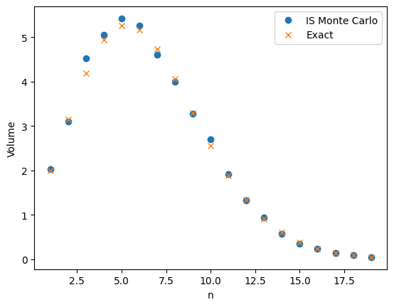
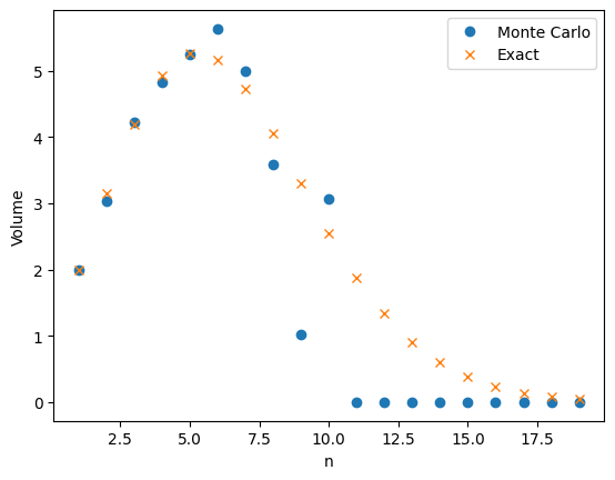
My last post was about using importance sampling to estimate the volume of high-dimensional ball. The two figures below compare plain Monte Carlo to using importance sampling with a Gaussian proposal. Both plots use \(M=1,000\) samples to estimate \(v_n\), the volume of an \(n\)-dimensional ball

A friend of mine pointed out that the relative error does not seem to increase with the dimension \(n\). He thought it was too good to be true. It turns out he was right and the relative error does increase with dimension but it increases very slowly. To estimate \(v_n\) the number of samples needs to grow on the order of \(\sqrt{n}\).

To prove this, we will use the paper The sample size required for importance sampling by Chatterjee and Diaconis [1]. This paper shows that the sample size for importance sampling is determined by the Kullback-Liebler divergence. The relevant result from their paper is Theorem 1.3. This theorem is about the relative error in using importance sampling to estimate a probability.

In our setting the proposal distribution is \(Q=\mathcal{N}(0,\frac{1}{n}I_n)\). That is the distribution \(Q\) is an \(n\)-dimensional Gaussian vector with mean \(0\) and covariance \(\frac{1}{n}I_n\). The conditional target distribution is \(P\) the uniform distribution on the \(n\) dimensional ball. Theorem 1.3 in [1] tells us how many samples are needed to estimate \(v_n\). Informally, the required sample size is \(M = O(\exp(D(P \Vert Q)))\). Here \(D(P\Vert Q)\) is the Kullback-Liebler divergence between \(P\) and \(Q\).

To use this theorem we need to compute \(D(P \Vert Q)\). Kullback-Liebler divergence is defined as integral. Specifically

\(\displaystyle{D(P\Vert Q) = \int_{\mathbb{R}^n} \log\frac{P(x)}{Q(x)}P(x)dx}\)

Computing the high-dimensional integral above looks challenging. Fortunately, it can reduced to a one-dimensional integral. This is because both the distributions \(P\) and \(Q\) are rotationally symmetric. To use this, define \(P_r,Q_r\) to be the distribution of the norm squared under \(P\) and \(Q\). That is if \(X \sim P\), then \(\Vert X \Vert_2^2 \sim P_R\) and likewise for \(Q_R\). By the rotational symmetry of \(P\) and \(Q\) we have

\(D(P\Vert Q) = D(P_R \Vert Q_R).\)

We can work out both \(P_R\) and \(Q_R\). The distribution \(P\) is the uniform distribution on the \(n\)-dimensional ball. And so for \(X \sim P\) and any \(r \in [0,1]\)

\(\mathbb{P}(\Vert X \Vert_2^2 \le r) = \frac{v_n r^n}{v_n} = r^n.\)

Which implies that \(P_R\) has density \(P_R(r)=nr^{n-1}\). This means that \(P_R\) is a Beta distribution with parameters \(\alpha = n, \beta = 1\). The distribution \(Q\) is a multivariate Gaussian distribution with mean \(0\) and variance \(\frac{1}{n}I_n\). This means that if \(X \sim Q\), then \(\Vert X \Vert_2^2 = \sum_{i=1}^n X_i^2\) is a scaled chi-squared variable. The shape parameter of \(Q_R\) is \(n\) and scale parameter is \(1/n\). The density for \(Q_R\) is therefor

\(Q_R(r) = \frac{n^{n/2}}{2^{n/2}\Gamma(n/2)}r^{n/2-1}e^{-nx/2}\)

The Kullback-Leibler divergence between \(P\) and \(Q\) is therefor

\(\displaystyle{D(P\Vert Q)=D(P_R\Vert Q_R) = \int_0^1 \log \frac{P_R(r)}{Q_R(r)} P_R(r)dr}\)

Getting Mathematica to do the above integral gives

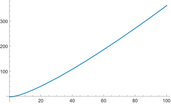
\(D(P \Vert Q) = -\frac{1+2n}{2+2n} + \frac{n}{2}\log(2 e) – (1-\frac{n}{2})\log n + \log \Gamma(\frac{n}{2}).\)

Using the approximation \(\log \Gamma(z) \approx (z-\frac{1}{2})\log(z)-z+O(1)\) we get that for large \(n\)

\(D(P \Vert Q) = \frac{1}{2}\log n + O(1)\).

And so the required number of samples is \(O(\exp(D(P \Vert Q)) = O(\sqrt{n}).\)

[1] Chatterjee, Sourav, and Persi Diaconis. “The sample size required in importance sampling.” The Annals of Applied Probability 28, no. 2 (2018): 1099–1135. https://www.jstor.org/stable/26542331. (Public preprint here https://arxiv.org/abs/1511.01437)

Auxiliary variables sampler

The auxiliary variables sampler is a general Markov chain Monte Carlo (MCMC) technique for sampling from probability distributions with unknown normalizing constants [1, Section 3.1]. Specifically, suppose we have \(n\) functions \(f_i : \mathcal{X} \to (0,\infty)\) and we want to sample from the probability distribution \(P(x) \propto \prod_{i=1}^n f_i(x).\) That is

\(\displaystyle{ P(x) = \frac{1}{Z}\prod_{i=1}^n f_i(x)},\)

where \(Z = \sum_{x \in \mathcal{X}} \prod_{i=1}^n f_i(x)\) is a normalizing constant. If the set \(\mathcal{X}\) is very large, then it may be difficult to compute \(Z\) or sample from \(P(x)\). To approximately sample from \(P(x)\) we can run an ergodic Markov chain with \(P(x)\) as a stationary distribution. Adding auxiliary variables is one way to create such a Markov chain. For each \(i \in \{1,\ldots,n\}\), we add a auxiliary variable \(U_i \ge 0\) such that

\(\displaystyle{P(U \mid X) = \prod_{i=1}^n \mathrm{Unif}[0,f_i(X)]}.\)

That is, conditional on \(X\), the auxiliary variables \(U_1,\ldots,U_n\) are independent and \(U_i\) is uniformly distributed on the interval \([0,f_i(X)]\). If \(X\) is distributed according to \(P\) and \(U_1,\ldots,U_n\) have the above auxiliary variable distribution, then

\(\displaystyle{P(X,U) =P(X)P(U\mid X)\propto \prod_{i=1}^n f_i(X) \frac{1}{f_i(X)} I[U_i \le f(X_i)] = \prod_{i=1}^n I[U_i \le f(X_i)]}.\)

This means that the joint distribution of \((X,U)\) is uniform on the set

\(\widetilde{\mathcal{X}} = \{(x,u) \in \mathcal{X} \times (0,\infty)^n : u_i \le f(x_i) \text{ for all } i\}.\)

Put another way, suppose we could jointly sample \((X,U)\) from the uniform distribution on \(\widetilde{\mathcal{X}}\). Then, the above calculation shows that if we discard \(U\) and only keep \(X\), then \(X\) will be sampled from our target distribution \(P\).

The auxiliary variables sampler approximately samples from the uniform distribution on \(\widetilde{\mathcal{X}}\) is by using a Gibbs sampler. The Gibbs samplers alternates between sampling \(U’\) from \(P(U \mid X)\) and then sampling \(X’\) from \(P(X \mid U’)\). Since the joint distribution of \((X,U)\) is uniform on \(\widetilde{\mathcal{X}}\), the conditional distributions \(P(X \mid U)\) and \(P(U \mid X)\) are also uniform. The auxiliary variables sampler thus transitions from \(X\) to \(X’\) according to the two step process

  1. Independently sample \(U_i\) uniformly from \([0,f_i(X)]\).
  2. Sample \(X’\) uniformly from the set \(\{x \in \mathcal{X} : f_i(x) \ge u_i \text{ for all } i\}\).

Since the auxiliary variables sampler is based on a Gibbs sampler, we know that the joint distribution of \((X,U)\) will converge to the uniform distribution on \(\mathcal{X}\). So when we discard \(U\), the distribution of \(X\) will converge to the target distribution \(P\)!

Auxiliary variables in practice

To perform step 2 of the auxiliary variables sampler we have to be able to sample uniformly from the sets

\(\mathcal{X}_u = \{x \in \mathcal{X}:f_i(x) \ge u_i \text{ for all } i\}. \)

Depending on the nature of the set \(\mathcal{X}\) and the functions \(f_i\), it might be difficult to do this. Fortunately, there are some notable examples where this step has been worked out. The very first example of auxiliary variables is the Swendsen-Wang algorithm for sampling from the Ising model [2]. In this model it is possible to sample uniformly from \(\mathcal{X}_u\). Another setting where we can sample exactly is when \(\mathcal{X}\) is the real numbers \(\mathcal{R}\) and each \(f_i\) is an increasing function of \(x\). This is explored in [3] where they apply auxiliary variables to sampling from Bayesian posteriors.

There is an alternative to sampling exactly from the uniform distribution on \(\mathcal{X}_u\). Instead of sampling \(X’\) uniformly from \(\mathcal{X}_u\), we can run a Markov chain from the old \(X\) that has the uniform distribution as a stationary distribution. This approach leads to another special case of auxiliary variables which is called “slice sampling” [4].

References

[1] Andersen HC, Diaconis P. Hit and run as a unifying device. Journal de la societe francaise de statistique & revue de statistique appliquee. 2007;148(4):5-28. http://www.numdam.org/item/JSFS_2007__148_4_5_0/
[2] Swendsen RH, Wang JS. Nonuniversal critical dynamics in Monte Carlo simulations. Physical review letters. 1987 Jan 12;58(2):86. https://journals.aps.org/prl/abstract/10.1103/PhysRevLett.58.86
[3] Damlen P, Wakefield J, Walker S. Gibbs sampling for Bayesian non‐conjugate and hierarchical models by using auxiliary variables. Journal of the Royal Statistical Society: Series B (Statistical Methodology). 1999 Apr;61(2):331-44. https://rss.onlinelibrary.wiley.com/doi/abs/10.1111/1467-9868.00179
[4] Neal RM. Slice sampling. The annals of statistics. 2003 Jun;31(3):705-67. https://projecteuclid.org/journals/annals-of-statistics/volume-31/issue-3/Slice-sampling/10.1214/aos/1056562461.full

Log-sum-exp trick with negative numbers

Suppose you want to calculate an expression of the form

\(\displaystyle{\log\left(\sum_{i=1}^n \exp(a_i) – \sum_{j=1}^m \exp(b_j)\right)},\)

where \(\sum_{i=1}^n \exp(a_i) > \sum_{j=1}^m \exp(b_j)\). Such expressions can be difficult to evaluate directly since the exponentials can easily cause overflow errors. In this post, I’ll talk about a clever way to avoid such errors.

If there were no terms in the second sum we could use the log-sum-exp trick. That is, to calculate

\(\displaystyle{\log\left(\sum_{i=1}^n \exp(a_i) \right)},\)

we set \(a=\max\{a_i : 1 \le i \le n\}\) and use the identity

\(\displaystyle{a + \log\left(\sum_{i=1}^n \exp(a_i-a)\right) = \log\left(\sum_{i=1}^n \exp(a_i)\right)}. \)

Since \(a_i \le a\) for all \(i =1,\ldots,n\), the left hand side of the above equation can be computed without the risk of overflow. To calculate,

\(\displaystyle{\log\left(\sum_{i=1}^n \exp(a_i) – \sum_{j=1}^m \exp(b_j)\right)},\)

we can use the above method to separately calculate

\(\displaystyle{A = \log\left(\sum_{i=1}^n \exp(a_i) \right)}\) and \(\displaystyle{B = \log\left(\sum_{j=1}^m \exp(b_j)\right)}.\)

The final result we want is \(\log\left(\sum_{i=1}^n \exp(a_i) – \sum_{j=1}^m \exp(b_j) \right)\) which is equal to

\(\displaystyle{ \log(\exp(A) – \exp(B)) = A + \log(1-\exp(B-A))}.\)

Since \(A > B\), the right hand side of the above expression can be evaluated safely and we will have our final answer.

R code

The R code below defines a function that performs the above procedure

# Safely compute log(sum(exp(pos)) - sum(exp(neg)))
# The default value for neg is an empty vector.

logSumExp <- function(pos, neg = c()){
  max_pos <- max(pos)
  A <- max_pos + log(sum(exp(pos - max_pos)))
  
  # If neg is empty, the calculation is done
  if (length(neg) == 0){
    return(A)
  }
  
  # If neg is non-empty, calculate B.
  max_neg <- max(neg)
  B <- max_neg + log(sum(exp(neg - max_neg)))
  
  # Check that A is bigger than B
  if (A <= B) {
    stop("sum(exp(pos)) must be larger than sum(exp(neg))")
  }
  
  # log1p() is a built in function that accurately calculates log(1+x) for |x| << 1
  return(A + log1p(-exp(B - A)))
}

An example

The above procedure can be used to evaulate

\(\displaystyle{\log\left(\sum_{i=1}^{200} i! – \sum_{i=1}^{500} \binom{500}{i}^2\right)}.\)

Evaluating this directly would quickly lead to errors since R (and most other programming languages) cannot compute \(200!\). However, R has the functions lfactorial() and lchoose() which can compute \(\log(i!)\) and \(\log\binom{n}{i}\) for large values of \(i\) and \(n\). We can thus put this expression in the general form at the start of this post

\(\displaystyle{\log\left(\sum_{i=1}^{200} \exp(\log(i!)) – \sum_{i=1}^{500} \exp\left(2\log\binom{500}{i}\right)\right)}.\)

The following R code thus us exactly what we want:

pos <- sapply(1:200, lfactorial)
neg <- sapply(1:500, function(i){2*lchoose(500, i)})

logSumExp(pos, neg)
# 863.237

The beta-binomial distribution

The beta-binomial model is a Bayesian model used to analyze rates. For a great derivation and explanation of this model, I highly recommend watching the second lecture from Richard McElreath’s course Statistical Rethinking. In this model, the data, \(X\), is assumed to be binomially distributed with a fixed number of trail \(N\) but an unknown rate \(\rho \in [0,1]\). The rate \(\rho\) is given a \(\text{Beta}(a,b)\) prior. That is the prior distribution of \(\rho\) has a density

\(p(\rho) = \frac{1}{B(a,b)} \rho^{a-1}(1-\rho)^{b-1},\)

where \(B(a,b) =\int_0^1 \rho^{a-1}(1-\rho)^{b-1}d\rho\) is a normalizing constant. The model can thus be written as

\(\rho \sim \text{Beta}(a,b),\)
\(X | \rho \sim \text{Binom}(N,\rho).\)

This is a conjugate model, meaning that the posterior distribution of \(\rho\) is again a beta distribution. This can be seen by using Bayes rule

\(p(\rho | X) \propto p(X| \rho)p(\rho) \propto \rho^{X+a-1}(1-\rho)^{(N-X)+b-1}.\)

The last expression is proportional to a beta density., specifically \(\rho | X \sim \text{Beta}(X+a, N-X+b)\).

The marginal distribution of \(X\)

In the above model we are given the distribution of \(\rho\) and the conditional distribution of \(X|\rho\). To calculate the distribution of \(X\), we thus need to marginalize over \(\rho\). Specifically,

\(\displaystyle{p(X) = \int_0^1 p(X,\rho)d\rho = \int_0^1 p(X| \rho)p(\rho)d\rho.}\)

The term inside the above integral is

\(\displaystyle{p(X| \rho)p(\rho) = \binom{N}{X}\rho^X(1-\rho)^{N-X}\frac{1}{B(a,b)}\rho^{a-1}(1-\rho)^{b-1} },\)

which is equal to \(\frac{\binom{N}{X}}{B(a,b)}\rho^{X+a-1}(1-\rho)^{N-X+b-1}\) and

\(\displaystyle{\int_0^1 \rho^{X+a-1}(1-\rho)^{N-X+b-1}d\rho=B(X+a, N-X+a)}\)

Thus,

\(\displaystyle{p(X) = \binom{N}{X}\frac{B(X+a, N-X+a)}{B(a,b)}}.\)

This distribution is called the beta-binomial distribution. Below is an image from Wikipedia showing a graph of \(p(X)\) for \(N=10\) and a number of different values of \(a\) and \(b\). You can see that, especially for small value of \(a\) and \(b\) the distribution is a lot more spread out than the binomial distribution. This is because there is randomness coming from both \(\rho\) and the binomial conditional distribution.

A plot of the beta-binomial distribution for different values of the parameters a and b. For small values of a and b, the distribution is very spread out.

Two sample tests as correlation tests

Suppose we have two samples \(Y_1^{(0)}, Y_2^{(0)},\ldots, Y_{n_0}^{(0)}\) and \(Y_1^{(1)},Y_2^{(1)},\ldots, Y_{n_1}^{(1)}\) and we want to test if they are from the same distribution. Many popular tests can be reinterpreted as correlation tests by pooling the two samples and introducing a dummy variable that encodes which sample each data point comes from. In this post we will see how this plays out in a simple t-test.

The equal variance t-test

In the equal variance t-test, we assume that \(Y_i^{(0)} \stackrel{\text{iid}}{\sim} \mathcal{N}(\mu_0,\sigma^2)\) and \(Y_i^{(1)} \stackrel{\text{iid}}{\sim} \mathcal{N}(\mu_1,\sigma^2)\), where \(\sigma^2\) is unknown. Our hypothesis that \(Y_1^{(0)}, Y_2^{(0)},\ldots, Y_{n_0}^{(0)}\) and \(Y_1^{(1)},Y_2^{(1)},\ldots, Y_{n_1}^{(1)}\) are from the same distribution becomes the hypothesis \(\mu_0 = \mu_1\). The test statistic is

\(t = \frac{\displaystyle \overline{Y}^{(1)} – \overline{Y}^{(0)}}{\displaystyle \hat{\sigma}\sqrt{\frac{1}{n_0}+\frac{1}{n_1}}}\),

where \(\overline{Y}^{(0)}\) and \(\overline{Y}^{(1)}\) are the two sample means. The variable \(\hat{\sigma}\) is the pooled estimate of the standard deviation and is given by

\(\hat{\sigma}^2 = \displaystyle\frac{1}{n_0+n_1-2}\left(\sum_{i=1}^{n_0}\left(Y_i^{(0)}-\overline{Y}^{(0)}\right)^2 + \sum_{i=1}^{n_1}\left(Y_i^{(1)}-\overline{Y}^{(1)}\right)^2\right)\).

Under the null hypothesis, \(t\) follows the T-distribution with \(n_0+n_1-2\) degrees of freedom. We thus reject the null \(\mu_0=\mu_1\) when \(|t|\) exceeds the \(1-\alpha/2\) quantile of the T-distribution.

Pooling the data

We can turn this two sample test into a correlation test by pooling the data and using a linear model. Let \(Y_1,\ldots,Y_{n_0}, Y_{n_0+1},\ldots,Y_{n_0+n_1}\) be the pooled data and for \(i = 1,\ldots, n_0+n_1\), define \(x_i \in \{0,1\}\) by

\(x_i = \begin{cases} 0 & \text{if } 1 \le i \le n_0,\\ 1 & \text{if } n_0+1 \le i \le n_0+n_1.\end{cases}\)

The assumptions that \(Y_i^{(0)} \stackrel{\text{iid}}{\sim} \mathcal{N}(\mu_0,\sigma^2)\) and \(Y_i^{(1)} \stackrel{\text{iid}}{\sim} \mathcal{N}(\mu_1,\sigma^2)\) can be rewritten as

\(Y_i = \beta_0+\beta_1x_i + \varepsilon_i,\)

where \(\varepsilon_i \stackrel{\text{iid}}{\sim} \mathcal{N}(0,\sigma^2)\). That is, we have expressed our modelling assumptions as a linear model. When working with this linear model, the hypothesis \(\mu_0 = \mu_1\) is equivalent to \(\beta_1 = 0\). To test \(\beta_1 = 0\) we can use the standard t-test for a coefficient in linear model. The test statistic in this case is

\(t’ = \displaystyle\frac{\hat{\beta}_1}{\hat{\sigma}_{OLS}\sqrt{(X^TX)^{-1}_{11}}},\)

where \(\hat{\beta}_1\) is the ordinary least squares estimate of \(\beta_1\), \(X \in \mathbb{R}^{(n_0+n_1)\times 2}\) is the design matrix and \(\hat{\sigma}_{OLS}\) is an estimate of \(\sigma\) given by

\(\hat{\sigma}_{OLS}^2 = \displaystyle\frac{1}{n_0+n_1-2}\sum_{i=1}^{n_0+n_1} (Y_i-\hat{Y}_i)^2,\)

where \(\hat{Y} = \hat{\beta}_0+\hat{\beta}_1x_i\) is the fitted value of \(Y_i\).

It turns out that \(t’\) is exactly equal to \(t\). We can see this by writing out the design matrix and calculating everything above. The design matrix has rows \([1,x_i]\) and is thus equal to

\(X = \begin{bmatrix} 1&x_1\\ 1&x_2\\ \vdots&\vdots\\ 1&x_{n_0}\\ 1&x_{n_0+1}\\ \vdots&\vdots\\ 1&x_{n_0+n_1}\end{bmatrix} = \begin{bmatrix} 1&0\\ 1&0\\ \vdots&\vdots\\ 1&0\\ 1&1\\ \vdots&\vdots\\ 1&1\end{bmatrix}.\)

This implies that

\(X^TX = \begin{bmatrix} n_0+n_1 &n_1\\n_1&n_1 \end{bmatrix},\)

And therefore,

\((X^TX)^{-1} = \frac{1}{(n_0+n_1)n_1-n_1^2}\begin{bmatrix} n_1 &-n_1\\-n_1&n_0+n_1 \end{bmatrix} =\begin{bmatrix} \frac{1}{n_0}&-\frac{1}{n_0}\\-\frac{1}{n_0}&\frac{1}{n_0}+\frac{1}{n_1}\end{bmatrix} .\)

Thus, \((X^TX)^{-1}_{11} = \frac{1}{n_0}+\frac{1}{n_1}\). So,

\(t’ = \displaystyle\frac{\hat{\beta}_1}{\hat{\sigma}_{OLS}\sqrt{\frac{1}{n_0}+\frac{1}{n_1}}},\)

which is starting to like \(t\) from the two-sample test. Now

\(X^TY = \begin{bmatrix} \displaystyle\sum_{i=1}^{n_0+n_1} Y_i\\ \displaystyle \sum_{i=n_0+1}^{n_0+n_1} Y_i \end{bmatrix} = \begin{bmatrix} n_0\overline{Y}^{(0)} + n_1\overline{Y}^{(1)}\\ n_1\overline{Y}^{(1)} \end{bmatrix}.\)

And so

\(\hat{\beta} = (X^TX)^{-1}X^TY =\begin{bmatrix} \overline{Y}^{(0)}\\ \overline{Y}^{(1)} -\overline{Y}^{(0)}\end{bmatrix}.\)

Thus, \(\hat{\beta}_1 = \overline{Y}^{(1)} -\overline{Y}^{(0)}\) and

\(t’ = \displaystyle\frac{\overline{Y}^{(1)}-\overline{Y}^{(0)}}{\hat{\sigma}_{OLS}\sqrt{\frac{1}{n_0}+\frac{1}{n_1}}}.\)

This means to show that \(t’ = t\), we only need to show that \(\hat{\sigma}_{OLS}^2=\hat{\sigma}^2\). To do this, note that the fitted values \(\hat{Y}\) are equal to

\(\displaystyle\hat{Y}_i=\hat{\beta}_0+x_i\hat{\beta}_1 = \begin{cases} \overline{Y}^{(0)} & \text{if } 1 \le i \le n_0,\\ \overline{Y}^{(1)} & \text{if } n_0+1\le i \le n_0+n_1\end{cases}.\)

Thus, \(\hat{\sigma}^2_{OLS} = \displaystyle\frac{1}{n_0+n_1-2}\sum_{i=1}^{n_0+n_1}\left(Y_i-\hat{Y}_i\right)^2\) is equal to

\(\displaystyle\frac{1}{n_0+n_1-2}\left(\sum_{i=1}^{n_0}\left(Y_i^{(0)}-\overline{Y}^{(0)}\right)^2 + \sum_{i=1}^{n_1}\left(Y_i^{(1)}-\overline{Y}^{(1)}\right)^2\right),\)

Which is exactly \(\hat{\sigma}^2\). Therefore, \(t’=t\) and the two sample t-test is equivalent to a correlation test.

The Friedman-Rafsky test

In the above example, we saw that the two sample t-test was a special case of the t-test for regressions. This is neat but both tests make very strong assumptions about the data. However, the same thing happens in a more interesting non-parametric setting.

In their 1979 paper, Jerome Friedman and Lawrence Rafsky introduced a two sample tests that makes no assumptions about the distribution of the data. The two samples do not even have to real-valued and can instead be from any metric space. It turns out that their test is a special case of another procedure they devised for testing for association (Friedman & Rafsky, 1983). As with the t-tests above, this connection comes from pooling the two samples and introducing a dummy variable.

I plan to write a follow up post explaining these procedures but you can also read about it in Chapter 6 of Group Representations in Probability and Statistics by Persi Diaconis.

References

Persi Diaconis “Group representations in probability and statistics,” pp 104-106, Hayward, CA: Institute of Mathematical Statistics, (1988)

Jerome H. Friedman, Lawrence C. Rafsky “Multivariate Generalizations of the Wald-Wolfowitz and Smirnov Two-Sample Tests,” The Annals of Statistics, Ann. Statist. 7(4), 697-717, (July, 1979)

Jerome H. Friedman, Lawrence C. Rafsky “Graph-Theoretic Measures of Multivariate Association and Prediction,” The Annals of Statistics, Ann. Statist. 11(2), 377-391, (June, 1983).