statistics – mathstoshare

Logistic regression with aggregate data

Logistic regression is a technique for analyzing data where the dependent variable is binary. In this post, we will introduce logistic regression and then discuss how to fit a logistic regression model using only aggregated count data.

Logistic regression overview

Logistic regression can be used when the dependent variable \(Y_i\) is binary. For example, in a medical study the dependent variable might be whether or not a patient developed a disease. In this case \(Y_i=1\) will mean that patient \(i\) did develop the disease and \(Y_i=0\) will mean that that patient \(i\) did not develop the disease. In logistic regression, the independent variables can either be categorical or quantitative. In the medical example, the type of treatment received could be a categorical independent variable and the age of the patient could be a quantitative independent variable.

Logistic regression models the probability that \(Y_i=1\) given the independent variables. If \(X_{i,1},\ldots,X_{p,1}\) are the values of the independent variables for patient \(i\), then logistic regression assumes that

\(\mathrm{Pr}(Y_i=1) = \sigma(\beta_0 + \beta_1 X_{i,1} + \cdots +\beta_p X_{i,p}) \),

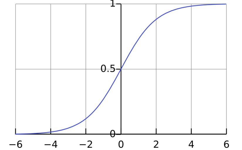
where \(\mathrm{Pr}(Y_i=1)\) is the probability that \(Y_i = 1\), \(\sigma\) is the logistic function \(\sigma(x) = \frac{1}{1+\exp(-x)}\) and \(\beta_0,\beta_1,\ldots,\beta_p\) are parameters that will be estimated from the data. The interpretation of the parameter \(\beta_j\) is that if \(X_{i,j}\) increases by 1 unit and all the other independent variables are fixed, then the odds \(\frac{\mathrm{Pr}(Y_i=1)}{\mathrm{Pr}(Y_i=0)}\) will increase by a factor of \(\exp(\beta_j)\).

Logistic regression models can be fit to data in using the function glm() in the programming language R. For example, to fit a logistic regression model with dependent variable disease and independent variables treatment and age, you can use the code

logistic_model <- glm(
          disease ~ treatment + age, 
          data = data, 
          family = binomial)

To view the estimates of the parameters of the model (as well as standard errors and p-values), you can run the code summary(logistic_model).

Logistic regression with aggregate data

If all of the independent variables are categorical, then it is possible to fit a logistic model with the aggregate count data. For example, the table below is from a study from the 1980s/1990s on the effect of AZT treatment on slowing the development of AIDS.¹

Race	AZT use	Symptoms	No Symptoms
Black	Yes	11	52
Black	No	12	43
White	Yes	14	93
White	No	32	81

The study featured 338 veterans who were positive for HIV and were beginning to show signs of faltering immune systems. The veterans were randomly assigned to either immediately receive AZT or to receive AZT once their T-cells showed signs of severe immune weakness. The table records whether the veterans received AZT immediately, the race of the veterans and whether they developed AIDS in the three year study period.

The table above shows aggregated data. The table reports the number of people for each combination of treatment, race and disease status. The table does not report individual patient data. However, it is it possible to fit a logistic regression model to the aggregate data.² We just need to make some small changes to the R code.

To describe the changes, let’s first review what we would do with the patient level data. Suppose we had a dataset individual_data that had a row for each veteran and had columns race, azt_use and developed_symptoms that record the veteran’s race, AZT use and whether they developed symptoms. Our goal is to fit a logistic regression model where dependent variable \(Y_i\) is a binary variable with \(Y_i=1\) meaning that the patient did develop symptoms. The independent variables are race and AZT use. With the individual data, we could use the following:

individual_model <- glm(
    developed_symptoms ~ race + azt_use, 
    family = binomial, 
    data = individual_data)

Now suppose that we only have the aggregate data in a table called aggregate_data. This table has columns race, azt_use, symptoms and no_symptoms like the table presented above. To fit the logistic model with this data, there are two options.

The first option is to replace the independent variable developed_symptoms in the individual model with cbind(symptoms, no_symptoms). The function cbind creates a matrix with two columns recording the number of people with and without symptoms for each combination of race and AZT use. We also need to tell R to use the aggregate data. Here is the R code:

aggregate_model_1 <- glm(
    cbind(symptoms, no_symptoms) ~ race + azt_use, 
    family = binomial, 
    data = aggregate_data

The other option is to replace the independent variable developed_symptoms with the proportion of people who developed symptoms. To use this option, it is also necessary to compute the total number of people for each combination of race and AZT use. These totals are used as weights in the logistic regression. In the code below, we first compute the proportion and the total number of people and then fit the model.

aggregate_data$total <- aggregate_data$symptoms + aggregate_data$no_symptomsaggregate_data$proportion <- aggregate_data$symptoms / aggregate_data$total

aggregate_model_2 <- glm(
    proportion ~ race + azt_use, 
    family = binomial,    weights = total,    data = aggregate_data)

Results

Both aggregate_model_1 and aggregate_model_2 produce the exact same parameter estimates, standard errors and p-values. More importantly, if we had the individual data, individual_model would also have the same results. We can actually check this by “de-aggregating” the data. This involves making a dataset with, for example, 11 rows with race = "Black", azt_use = "Yes" and developed_symptoms = 1 so that these 11 rows represent the 11 veterans in the first category of the table above.

All three logisitic regression models give the same final results:

	Estimate	Standard error	p-value
Intercept	-1.07	0.263	4e-05
raceWhite	0.05	0.289	0.848
atz_useYes	-0.719	0.279	0.01

The parameter estimates shows that Black and White veterans had approximately the same chance of developing symptoms (assuming that they either both received ATZ treatment or that neither of them received ATZ treatment). On the other hand, the parameter estimate for ATZ use is significant. The estimated value of -0.719 can be interpreted as follows. If the race of the veteran is held constant, then the odds of developing symptoms was half as high for the veterans who immediately took ATZ than for those who waited. In mathematical symbols:

\(\frac{\mathrm{Pr}(\text{developed symptoms} \mid \text{ATZ immediately})}{\mathrm{Pr}(\text{did not develop symptoms} \mid \text{ATZ immediately})}\)

is roughly equal to

\( 0.5 \times \frac{\mathrm{Pr}(\text{developed symptoms} \mid \text{waited for ATZ use})}{\mathrm{Pr}(\text{did not develop symptoms} \mid \text{waited for ATZ})} \)

The specific value of 0.5 comes from the fact that \(\exp(-0.719) \approx 0.5\). Section 5.4.2 of Categorical Data Analysis by Alan Agresti discusses the interpretation of the parameter estimates for this example in more detail.

R code for fitting all three models is available at the end of this post.³

Footnotes

The data on AZT is from Table 5.6 of Alan Agresti’s Categorical Data Analysis (3rd edition) https://onlinelibrary.wiley.com/doi/book/10.1002/0471249688, https://mybiostats.wordpress.com/wp-content/uploads/2015/03/3rd-ed-alan_agresti_categorical_data_analysis.pdf ↩︎
In statistical jargon, the aggregate data are sufficient statistics for the logistic regression model. ↩︎
R code: ↩︎


# Aggregate data from Agresti Table 5.6
aggregate_data <- data.frame(
  race = c("Black", "Black", "White", "White"),
  atz_use = c("yes", "no", "yes", "no"),
  symptoms = c(11, 12, 14, 32),
  no_symptoms = c(52, 43, 93, 81)
)

# Aggregate model 1 using cbind()
aggregate_model_1 <- glm(
  cbind(symptoms, no_symptoms) ~ race + atz_use,
  data = aggregate_data,
  family = binomial)

# Aggregate model 2 using proportions and weights
aggregate_data$total <- aggregate_data$symptoms + aggregate_data$no_symptoms
aggregate_data$proportion <- aggregate_data$symptoms / aggregate_data$total

aggregate_model_2 <- glm(
  proportion ~ race + atz_use,
  data = aggregate_data,
  weights = total,
  family = binomial)

# Individual model

# Function to "de-aggregate"
deaggregate_data <- function(aggregate_data) {
  # Create an empty list to store rows
  rows_list <- list()
  
  # Iterate through each row of aggregate data
  for (i in 1:nrow(aggregate_data)) {
    race_val <- aggregate_data$race[i]
    atz_val <- aggregate_data$atz_use[i]
    n_symptoms <- aggregate_data$symptoms[i]
    n_no_symptoms <- aggregate_data$no_symptoms[i]
    
    # Create rows for those with symptoms
    if (n_symptoms > 0) {
      rows_list[[length(rows_list) + 1]] <- data.frame(
        race = rep(race_val, n_symptoms),
        atz_use = rep(atz_val, n_symptoms),
        developed_symptoms = rep(1, n_symptoms)
      )
    }
    
    # Create rows for those without symptoms
    if (n_no_symptoms > 0) {
      rows_list[[length(rows_list) + 1]] <- data.frame(
        race = rep(race_val, n_no_symptoms),
        atz_use = rep(atz_val, n_no_symptoms),
        developed_symptoms = rep(0, n_no_symptoms)
      )
    }
  }
  
  # Combine all rows into one data frame
  do.call(rbind, rows_list)
}

individual_data <- deaggregate_data(aggregate_data)

individual_model <- glm(
  developed_symptoms ~ race + atz_use,
  data = individual_data,
  family = binomial
)

# Compare models
summary(aggregate_model_1)
summary(aggregate_model_2)
summary(individual_model)

Poisson approximations to the negative binomial distribution

This post is an introduction to the negative binomial distribution and a discussion of different ways of approximating the negative binomial distribution.

The negative binomial distribution describes the number of times a coin lands on tails before a certain number of heads are recorded. The distribution depends on two parameters \(p\) and \(r\). The parameter \(p\) is the probability that the coin lands on heads and \(r\) is the number of heads. If \(X\) has the negative binomial distribution, then \(X = x\) means in the first \(x+r-1\) tosses of the coin, there were \(r-1\) heads and that toss number \(x+r\) was a head. This means that the probability that \(X=x\) is given by

\(\displaystyle{f(x) = \binom{x+r-1}{r-1}p^{r}\left(1-p\right)^x}\)

Here is a plot of the function \(f(x)\) for different values of \(r\) and \(p\).

Poisson approximations

When the parameter \(r\) is large and \(p\) is close to one, the negative binomial distribution can be approximated by a Poisson distribution. More formally, suppose that \(r(1-p)=\lambda\) for some positive real number \(\lambda\). If \(r\) is large then, the negative binomial random variable with parameters \(p\) and \(r\), converges to a Poisson random variable with parameter \(\lambda\). This is illustrated in the picture below where three negative binomial distributions with \(r(1-p)=5\) approach the Poisson distribution with \(\lambda =5\).

Total variation distance is a common way to measure the distance between two discrete probability distributions. The log-log plot below shows that the error from the Poisson approximation is on the order of \(1/r\) and that the error is bigger if the limiting value of \(r(1-p)\) is larger.

It turns out that is is possible to get a more accurate approximation by using a different Poisson distribution. In the first approximation, we used a Poisson random variable with mean \(\lambda = r(1-p)\). However, the mean of the negative binomial distribution is \(r(1-p)/p\). This suggests that we can get a better approximation by setting \(\lambda = r(1-p)/p\).

The change from \(\lambda = r(1-p)\) to \(\lambda = r(1-p)/p\) is a small because \(p \approx 1\). However, this small change gives a much better approximation, especially for larger values of \(r(1-p)\). The below plot shows that both approximations have errors on the order of \(1/r\), but the constant for the second approximation is much better.

Second order accurate approximation

It is possible to further improve the Poisson approximation by using a Gram–Charlier expansion. A Gram–Charlier approximation for the Poisson distribution is given in this paper.¹ The approximation is

\(\displaystyle{f_{GC}(x) = P_\lambda(x) – \frac{1}{2}q\left((x-\lambda)P_\lambda(x)-(x-1-\lambda)P_\lambda(x-1)\right)},\)

where \(\lambda = \frac{k(1-p)}{p}\), \(q=1-p\), and \(P_\lambda(x)\) is the Poisson pmf evaluated at \(x\).

The Gram–Charlier expansion is considerably more accurate than either Poisson approximation. The errors are on the order of \(1/r^2\). This higher accuracy means that the error curves for the Gram–Charlier expansion has a steeper slope.

The approximation is given in equation (4) of the paper and is stated in terms of the CDF instead of the PMF. The equation also contains a small typo, it should say \(\frac{1}{2}q\) instead of \(\frac{1}{2}p\). ↩︎

“Uniformly random”

The term “uniformly random” sounds like a contradiction. How can the word “uniform” be used to describe anything that’s random? Uniformly random actually has a precise meaning, and, in a sense, means “as random as possible.” I’ll explain this with an example about shuffling card.

Shuffling cards

Suppose I have a deck of ten cards labeled 1 through 10. Initially, the cards are face down and in perfect order. The card labeled 10 is on top of the deck. The card labeled 9 is second from the top, and so on down to the card labeled 1. The cards are definitely not random.

Next, I generate a random number between 1 and 10. I then find the card with the corresponding label and put it face down on top of the deck. The cards are now somewhat random. The number on top could anything, but the rest of the cards are still in order. The cards are random but they are not uniformly random.

Now suppose that I keep generating random numbers and moving cards to the top of the deck. Each time I do this, the cards get more random. Eventually (after about 30 moves¹) the cards will be really jumbled up. Even if you knew the first few cards, it would be hard to predict the order of the remaining ones. Once the cards are really shuffled, they are uniformly random.

Uniformly random

A deck of cards is uniformly random if each of the possible arrangements of the cards are equally likely. After only moving one card, the deck of cards is not uniformly random. This is because there are only 10 possible arrangements of the deck. Once the deck is well-shuffled, all of the 3,628,800 possible arrangements are equally likely.

In general, something is uniformly random if each possibility is equally likely. So the outcome of rolling a fair 6-sided die is uniformly random, but rolling a loaded die is not. The word “uniform” refers to the chance of each possibility (1/6 for each side of the die). These chances are all the same and “uniform”.

This is why uniformly random can mean “as random as possible.” If you are using a fair die or a well-shuffled deck, there are no biases in the outcome. Mathematically, this means you can’t predict the outcome.

Communicating research

The inspiration for this post came from a conversation I had earlier in the week. I was telling someone about my research. As an example, I talked about how long it takes for a deck of cards to become uniformly random. They quickly stopped me and asked how the two words could ever go together. It was a good point! I use the words uniformly random all the time and had never realized this contradiction.² It was a good reminder about the challenge of clear communication.

Footnotes

The number of moves it takes for the deck to well-shuffled is actually random. But on average it takes around 30 moves. For the mathematical details, see Example 1 in Shuffling Cards and Stopping Times by David Aldous and Persi Diaconis. ↩︎
Of the six posts I published last year, five contain the word uniform! ↩︎

Understanding the Ratio of Uniforms Distribution

The ratio of uniforms distribution is a useful distribution for rejection sampling. It gives a simple and fast way to sample from discrete distributions like the hypergeometric distribution¹. To use the ratio of uniforms distribution in rejection sampling, we need to know the distributions density. This post summarizes some properties of the ratio of uniforms distribution and computes its density.

The ratio of uniforms distribution is the distribution of the ratio of two independent uniform random variables. Specifically, suppose \(U \in [-1,1]\) and \(V \in [0,1]\) are independent and uniformly distributed. Then \(R = U/V\) has the ratio of uniforms distribution. The plot below shows a histogram based on 10,000 samples from the ratio of uniforms distribution².

The histogram has a flat section in the middle and then curves down on either side. This distinctive shape is called a “table mountain”. The density of \(R\) also has a table mountain shape.

And here is the density plotted on top of the histogram.

A formula for the density of \(R\) is

\[h(R) = \begin{cases} \frac{1}{4} & \text{if } -1 \le R \le 1, \\\frac{1}{4R^2} & \text{if } R < -1 \text{ or } R > 1.\end{cases}\]

The first case in the definition of \(h\) corresponds to the flat part of the table mountain. The second case corresponds to the sloping curves. The rest of this post use geometry to derive the above formula for \(h(R)\).

Calculating the density

The point \((U,V)\) is uniformly distributed in the box \(B=[-1,1] \times [0,1]\). The image below shows an example of a point \((U,V)\) inside the box \(B\).

We can compute the ratio \(R = U/V\) geometrically. First we draw a straight line that starts at \((0,0)\) and goes through \((U,V)\). This line will hit the horizontal line \(y=1\). The \(x\) coordinate at this point is exactly \(R=U/V\).

In the above picture, all of the points on the dashed line map to the same value of \(R\). We can compute the density of \(R\) by computing an area. The probability that \(R\) is in a small interval \([R,R+dR]\) is \(\frac{\text{Area}(\{(u,v) \in B : u/v \in [R, R+dR]\})}{\text{Area}(B)}\) which is equal to

\[\frac{1}{2}\text{Area}(\{(u,v) \in B : u/v \in [R, R+dR]\}).\]

If we can compute the above area, then we will know the density of \(R\) because by definition

\(\displaystyle{h(R) = \lim_{dR \to 0} \frac{1}{2dR}\text{Area}(\{(u,v) \in B : u/v \in [R, R+dR]\})}.\)

We will first work on the case when \(R\) is between \(-1\) and \(1\). In this case, the set \(\{(u,v) \in B : u/v \in [R, R+dR]\}\) is a triangle. This triangle is drawn in blue below.

The horizontal edge of this triangle has length \(dR\). The perpendicular height of the triangle from the horizontal edge is \(1\). This means that

\[\text{Area}(\{(u,v) \in B : u/v \in [R, R+dR]\}) =\frac{dR}{2}.\]

And so, when \(R \in [-1,1]\) we have

\(\displaystyle{h(R) = \lim_{dR\to 0} \frac{1}{2dR}\times \frac{dR}{2}=\frac{1}{4}}.\)

Now let’s work on the case when \(R\) is bigger than \(1\) or less than \(-1\). In this case, the set \(\{(u,v) \in B : u/v \in [R, R+dR]\}\) is again triangle. But now the triangle has a vertical edge and is much skinnier. Below the triangle is drawn in red. Note that only points inside the box \(B\) are coloured in.

The vertical edge of the triangle has length \(\frac{1}{R} – \frac{1}{R+dR}= \frac{dR}{R(R+dR)}\). The perpendicular height of the triangle from the vertical edge is \(1\). Putting this together

\(\displaystyle{\text{Area}(\{(u,v) \in B : u/v \in [R, R+dR]\}) =\frac{dR}{2R(R+dR)}}.\)

And so

\(\displaystyle{h(R) = \lim_{dR \to 0} \frac{1}{2dR} \times \frac{dR}{2 R(R+dR)} = \frac{1}{4R^2}}.\)

And so putting everything together

\(\displaystyle{h(R) = \begin{cases} \frac{1}{4} & \text{if } -1 \le R \le 1, \\\frac{1}{4R^2} & \text{if } R < -1 \text{ or } R > 1.\end{cases}}\)

Footnotes and references

https://ieeexplore.ieee.org/document/718718 ↩︎
For visual purposes, I restricted the sample to values of \(R\) between \(-8\) and \(8\). This is because the ratio of uniform distribution has heavy tails. This meant that there were some very large values of \(R\) that made the plot hard to see. ↩︎

The discrete arcsine distribution

The discrete arcsine distribution is a probability distribution on \(\{0,1,\ldots,n\}\). It is a u-shaped distribution. There are peaks at \(0\) and \(n\) and a dip in the middle. The figure below shows the probability distribution function for \(n=10,15, 20\).

The probability distribution function of the arcsine distribution is given by

\(\displaystyle{p_n(k) = \frac{1}{2^{2n}}\binom{2k}{k}\binom{2n-2k)}{n-k}\text{ for } k \in \{0,1,\ldots,n\}}\)

The discrete arcsine distribution is related to simple random walks and to an interesting Markov chain called the Burnside process. The connection with simple random walks is explained in Chapter 3, Volume 1 of An Introduction to Probability and its applications by William Feller. The connection to the Burnside process was discovered by Persi Diaconis in Analysis of a Bose-Einstein Markov Chain.

The discrete arcsine distribution gets its name from the continuous arcsine distribution. Suppose \(X_n\) is distributed according to the discrete arcsine distribution with parameter \(n\). Then the normalized random variables \(X_n/n\) converges in distribution to the continuous arcsine distribution on \([0,1]\). The continuous arcsine distribution has the probability density function

\(\displaystyle{f(x) = \frac{1}{\pi\sqrt{x(1-x)}} \text{ for } 0 \le x \le 1}\)

This means that continuous arcsine distribution is a beta distribution with \(\alpha=\beta=1/2\). It is called the arcsine distribution because the cumulative distribution function involves the arcsine function

\(\displaystyle{F(x) = \int_0^x f(y)dy = \frac{2}{\pi}\arcsin(\sqrt{x}) \text{ for } 0 \le x \le 1}\)

There is another connection between the discrete and continuous arcsine distributions. The continuous arcsine distribution can be used to sample the discrete arcsine distribution. The two step procedure below produces a sample from the discrete arcsine distribution with parameter \(n\):

Sample \(p\) from the continuous arcsine distribution.
Sample \(X\) from the binomial distribution with parameters \(n\) and \(p\).

This means that the discrete arcsine distribution is actually the beta-binomial distribution with parameters \(\alpha = \beta =1/2\). I was surprised when I was told this, and couldn’t find a reference. The rest of this blog post proves that the discrete arcsine distribution is an instance of the beta-binomial distribution.

As I showed in this post, the beta-binomial distribution has probability distribution function:

\(\displaystyle{q_{\alpha,\beta,n}(k) = \binom{n}{k}\frac{B(k+\alpha, n-k+\alpha)}{B(a,b)}},\)

where \(B(x,y)=\frac{\Gamma(x)\Gamma(y)}{\Gamma(x+y)}\) is the Beta-function. To show that the discrete arc sine distribution is an instance of the beta-binomial distribution we need that \(p_n(k)=q_{1/2,1/2,n}(k)\). That is

\(\displaystyle{ \binom{n}{k}\frac{B(k+1/2, n-k+1/2)}{B(1/2,1/2)} = \frac{1}{2^{2n}}\binom{2k}{k}\binom{2n-2k}{n-k}}\),

for all \(k = 0,1,\ldots,n\). To prove the above equation, we can first do some simplifying to \(q_{1/2,1/2,n}(k)\). By definition

\(\displaystyle{\frac{B(k+1/2, n-k+1/2)}{B(1/2,1/2)} = \frac{\frac{\Gamma(k+1/2)\Gamma(n-k+1/2)}{\Gamma(n+1)}}{\frac{\Gamma(1/2)\Gamma(1/2)}{\Gamma(1)}}}\),

Since \(\Gamma(m)=(m-1)!\) if \(m\) is a natural number this complicated fraction simplifies to

\[\frac{1}{n!}\frac{\Gamma(k+1/2)}{\Gamma(1/2)}\frac{\Gamma(n-k+1/2)}{\Gamma(1/2)}\]

The Gamma function \(\Gamma(x)\) also satisfies the property \(\Gamma(x+1)=x\Gamma(x)\). Using this repeatedly gives

\(\displaystyle{\Gamma(k+1/2) = (k-1/2) (k-3/2) \times \cdots \times \frac{3}{2}\times\frac{1}{2}\times\Gamma(1/2) }. \)

This means that

\(\displaystyle{\frac{\Gamma(k+1/2)}{\Gamma(1/2)} = (k-1/2) (k-3/2)\times \cdots \times \frac{3}{2}\times\frac{1}{2} =\frac{(2k-1)!!}{2^k}},\)

where \((2k-1)!!=(2k-1)\times (2k-3)\times\cdots \times 3 \times 1\) is the double factorial. The same reasoning gives

\(\displaystyle{\frac{\Gamma(n-k+1/2)}{\Gamma(1/2)} =\frac{(2n-2k-1)!!}{2^{n-k}}}.\)

And so

\(\displaystyle{q_{1/2,1/2,n}(k) =\frac{1}{2^nk!(n-k)!}(2k-1)!!(2n-2k-1)!!}.\)

We’ll now show that \(p_n(k)\) is also equal to the above final expression. Recall

\(\displaystyle{p_n(k) = \frac{1}{2^{2n}} \binom{2k}{k}\binom{2(n-k)}{n-k} = \frac{1}{2^{2n}}\frac{(2k)!(2(n-k))!}{k!k!(n-k)!(n-k)!} }.\)

By shuffling some of the terms

\[p_n(k)=\frac{1}{2^nk!(n-k)!}\frac{(2k)!}{k!2^k}\frac{(2n-2k)!}{(n-k)!2^{n-k}}\]

And so it suffices to show \(\frac{(2k)!}{k!2^k} = (2k-1)!!\) (and hence \(\frac{(2n-2k)!}{(n-k)!2^{n-k}}=(2n-2k-1)!!\)). To see why this last claim holds, note that

\(\displaystyle{\frac{(2k)!}{k!2^k} = \frac{(2k)(2k-1)(2k-2)\times\cdots\times 3 \times 2 \times 1}{(2k)(2k-2)\times \cdots \times 2} = (2k-1)!!}\)

Showing that \(p_{n}(k)=q_{n,1/2,1/2}(k)\) as claimed.