Tag: sampling

  • Understanding the Ratio of Uniforms Distribution

    The ratio of uniforms distribution is a useful distribution for rejection sampling. It gives a simple and fast way to sample from discrete distributions like the hypergeometric distribution1. To use the ratio of uniforms distribution in rejection sampling, we need to know the distributions density. This post summarizes some properties of the ratio of uniforms distribution and computes its density.

    The ratio of uniforms distribution is the distribution of the ratio of two independent uniform random variables. Specifically, suppose \(U \in [-1,1]\) and \(V \in [0,1]\) are independent and uniformly distributed. Then \(R = U/V\) has the ratio of uniforms distribution. The plot below shows a histogram based on 10,000 samples from the ratio of uniforms distribution2.
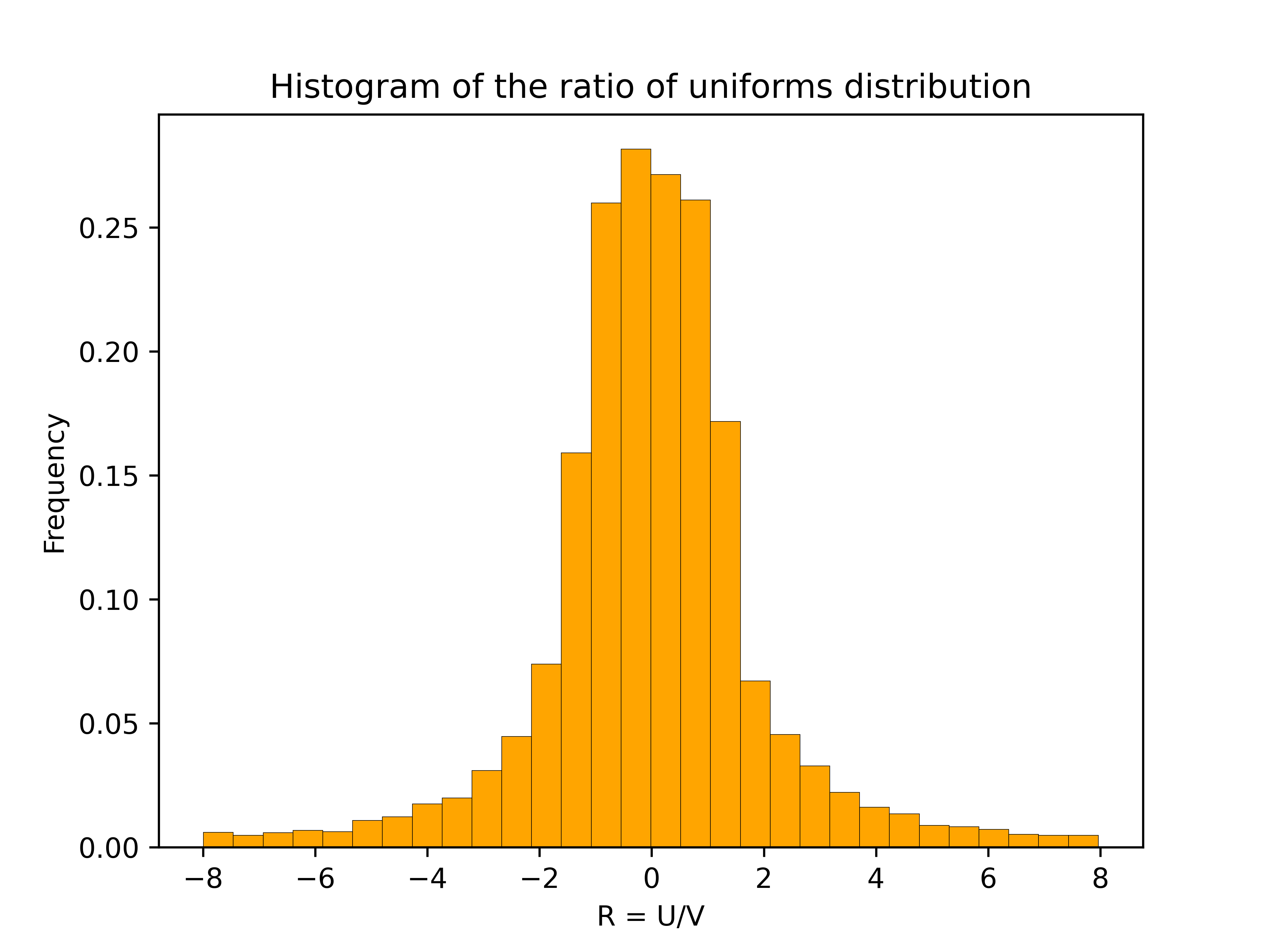
    The histogram has a flat section in the middle and then curves down on either side. This distinctive shape is called a “table mountain”. The density of \(R\) also has a table mountain shape.

    And here is the density plotted on top of the histogram.
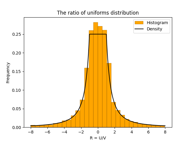
    A formula for the density of \(R\) is

    \(\displaystyle{h(R) = \begin{cases} \frac{1}{4} & \text{if } -1 \le R \le 1, \\\frac{1}{4R^2} & \text{if } R < -1 \text{ or } R > 1.\end{cases}}\)

    The first case in the definition of \(h\) corresponds to the flat part of the table mountain. The second case corresponds to the sloping curves. The rest of this post use geometry to derive the above formula for \(h(R)\).

    Calculating the density

    The point \((U,V)\) is uniformly distributed in the box \(B=[-1,1] \times [0,1]\). The image below shows an example of a point \((U,V)\) inside the box \(B\).
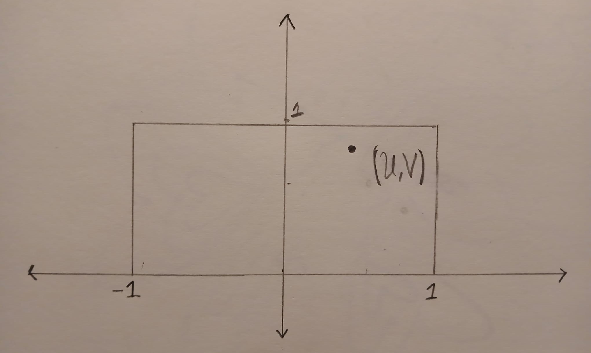
    We can compute the ratio \(R = U/V\) geometrically. First we draw a straight line that starts at \((0,0)\) and goes through \((U,V)\). This line will hit the horizontal line \(y=1\). The \(x\) coordinate at this point is exactly \(R=U/V\).
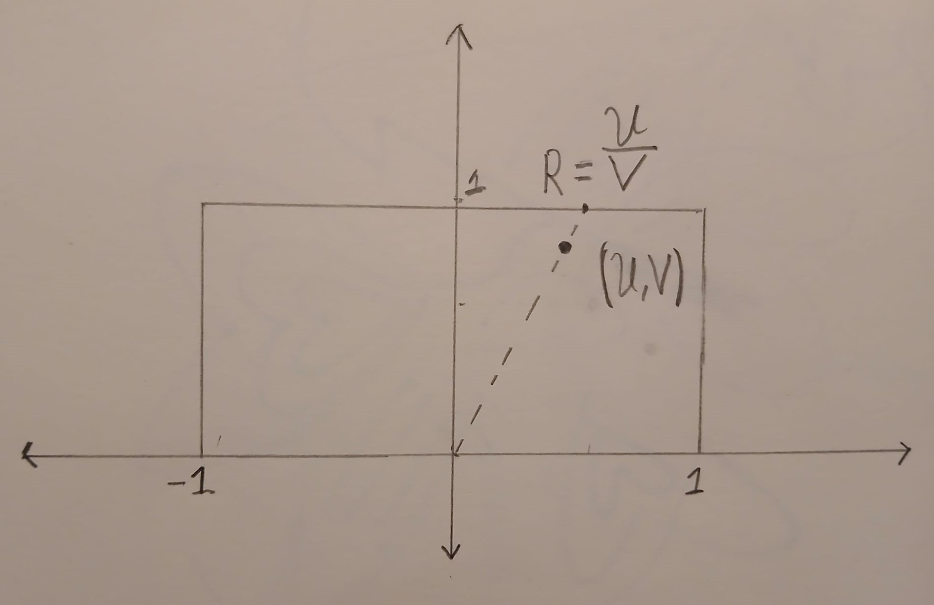
    In the above picture, all of the points on the dashed line map to the same value of \(R\). We can compute the density of \(R\) by computing an area. The probability that \(R\) is in a small interval \([R,R+dR]\) is

    \(\displaystyle{\frac{\text{Area}(\{(u,v) \in B : u/v \in [R, R+dR]\})}{\text{Area}(B)} = \frac{1}{2}\text{Area}(\{(u,v) \in B : u/v \in [R, R+dR]\}).}\)

    If we can compute the above area, then we will know the density of \(R\) because by definition

    \(\displaystyle{h(R) = \lim_{dR \to 0} \frac{1}{2dR}\text{Area}(\{(u,v) \in B : u/v \in [R, R+dR]\})}.\)

    We will first work on the case when \(R\) is between \(-1\) and \(1\). In this case, the set \(\{(u,v) \in B : u/v \in [R, R+dR]\}\) is a triangle. This triangle is drawn in blue below.
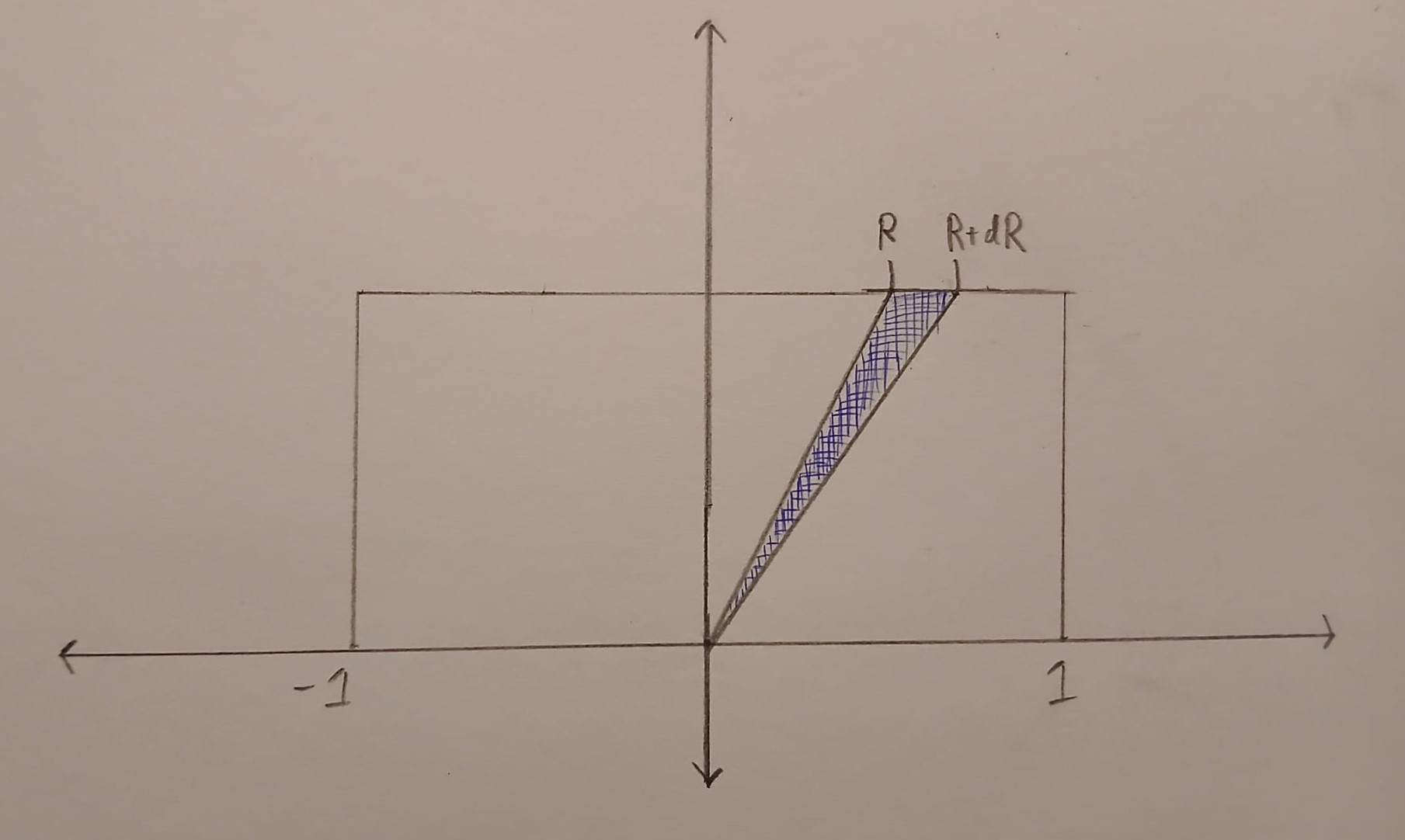
    The horizontal edge of this triangle has length \(dR\). The perpendicular height of the triangle from the horizontal edge is \(1\). This means that

    \( \displaystyle{\text{Area}(\{(u,v) \in B : u/v \in [R, R+dR]\}) =\frac{1}{2}\times dR \times 1=\frac{dR}{2}}.\)

    And so, when \(R \in [-1,1]\) we have

    \(\displaystyle{h(R) = \lim_{dR\to 0} \frac{1}{2dR}\times \frac{dR}{2}=\frac{1}{4}}.\)

    Now let’s work on the case when \(R\) is bigger than \(1\) or less than \(-1\). In this case, the set \(\{(u,v) \in B : u/v \in [R, R+dR]\}\) is again triangle. But now the triangle has a vertical edge and is much skinnier. Below the triangle is drawn in red. Note that only points inside the box \(B\) are coloured in.
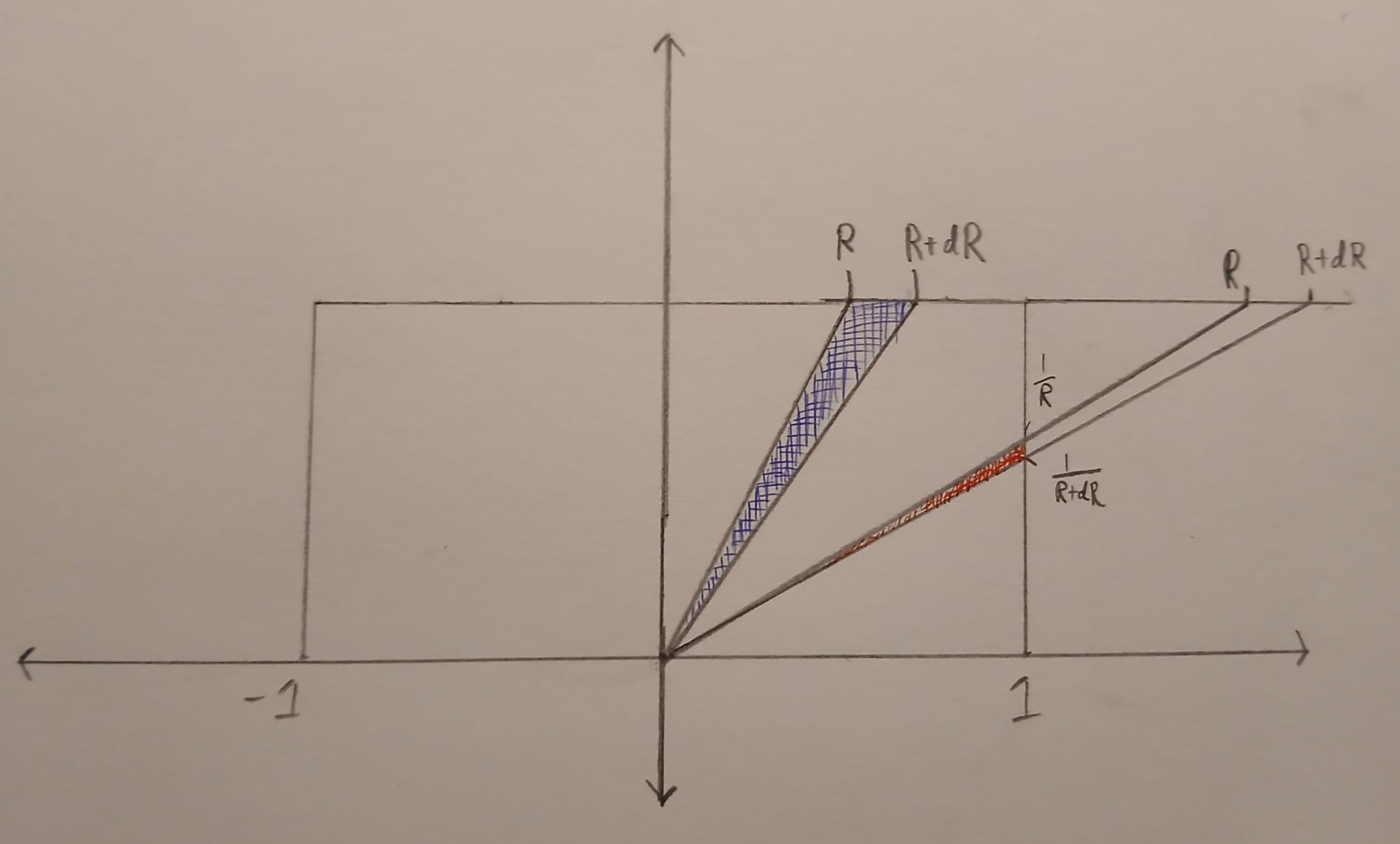
    The vertical edge of the triangle has length \(\frac{1}{R} – \frac{1}{R+dR}= \frac{dR}{R(R+dR)}\). The perpendicular height of the triangle from the vertical edge is \(1\). Putting this together

    \( \displaystyle{\text{Area}(\{(u,v) \in B : u/v \in [R, R+dR]\}) =\frac{1}{2}\times \frac{dR}{R(R+dR)} \times 1=\frac{dR}{2R(R+dR)}}.\)

    And so

    \(\displaystyle{h(R) = \lim_{dR \to 0} \frac{1}{2dR} \times \frac{dR}{2 R(R+dR)} = \frac{1}{4R^2}}.\)

    And so putting everything together

    \(\displaystyle{h(R) = \begin{cases} \frac{1}{4} & \text{if } -1 \le R \le 1, \\\frac{1}{4R^2} & \text{if } R < -1 \text{ or } R > 1.\end{cases}}\)

    Footnotes and references

    1. https://ieeexplore.ieee.org/document/718718 ↩︎
    2. For visual purposes, I restricted the sample to values of \(R\) between \(-8\) and \(8\). This is because the ratio of uniform distribution has heavy tails. This meant that there were some very large values of \(R\) that made the plot hard to see. ↩︎
  • Auxiliary variables sampler

    The auxiliary variables sampler is a general Markov chain Monte Carlo (MCMC) technique for sampling from probability distributions with unknown normalizing constants [1, Section 3.1]. Specifically, suppose we have \(n\) functions \(f_i : \mathcal{X} \to (0,\infty)\) and we want to sample from the probability distribution \(P(x) \propto \prod_{i=1}^n f_i(x).\) That is

    \(\displaystyle{ P(x) = \frac{1}{Z}\prod_{i=1}^n f_i(x)},\)

    where \(Z = \sum_{x \in \mathcal{X}} \prod_{i=1}^n f_i(x)\) is a normalizing constant. If the set \(\mathcal{X}\) is very large, then it may be difficult to compute \(Z\) or sample from \(P(x)\). To approximately sample from \(P(x)\) we can run an ergodic Markov chain with \(P(x)\) as a stationary distribution. Adding auxiliary variables is one way to create such a Markov chain. For each \(i \in \{1,\ldots,n\}\), we add a auxiliary variable \(U_i \ge 0\) such that

    \(\displaystyle{P(U \mid X) = \prod_{i=1}^n \mathrm{Unif}[0,f_i(X)]}.\)

    That is, conditional on \(X\), the auxiliary variables \(U_1,\ldots,U_n\) are independent and \(U_i\) is uniformly distributed on the interval \([0,f_i(X)]\). If \(X\) is distributed according to \(P\) and \(U_1,\ldots,U_n\) have the above auxiliary variable distribution, then

    \(\displaystyle{P(X,U) =P(X)P(U\mid X)\propto \prod_{i=1}^n f_i(X) \frac{1}{f_i(X)} I[U_i \le f(X_i)] = \prod_{i=1}^n I[U_i \le f(X_i)]}.\)

    This means that the joint distribution of \((X,U)\) is uniform on the set

    \(\widetilde{\mathcal{X}} = \{(x,u) \in \mathcal{X} \times (0,\infty)^n : u_i \le f(x_i) \text{ for all } i\}.\)

    Put another way, suppose we could jointly sample \((X,U)\) from the uniform distribution on \(\widetilde{\mathcal{X}}\). Then, the above calculation shows that if we discard \(U\) and only keep \(X\), then \(X\) will be sampled from our target distribution \(P\).

    The auxiliary variables sampler approximately samples from the uniform distribution on \(\widetilde{\mathcal{X}}\) is by using a Gibbs sampler. The Gibbs samplers alternates between sampling \(U’\) from \(P(U \mid X)\) and then sampling \(X’\) from \(P(X \mid U’)\). Since the joint distribution of \((X,U)\) is uniform on \(\widetilde{\mathcal{X}}\), the conditional distributions \(P(X \mid U)\) and \(P(U \mid X)\) are also uniform. The auxiliary variables sampler thus transitions from \(X\) to \(X’\) according to the two step process

    1. Independently sample \(U_i\) uniformly from \([0,f_i(X)]\).
    2. Sample \(X’\) uniformly from the set \(\{x \in \mathcal{X} : f_i(x) \ge u_i \text{ for all } i\}\).

    Since the auxiliary variables sampler is based on a Gibbs sampler, we know that the joint distribution of \((X,U)\) will converge to the uniform distribution on \(\mathcal{X}\). So when we discard \(U\), the distribution of \(X\) will converge to the target distribution \(P\)!

    Auxiliary variables in practice

    To perform step 2 of the auxiliary variables sampler we have to be able to sample uniformly from the sets

    \(\mathcal{X}_u = \{x \in \mathcal{X}:f_i(x) \ge u_i \text{ for all } i\}. \)

    Depending on the nature of the set \(\mathcal{X}\) and the functions \(f_i\), it might be difficult to do this. Fortunately, there are some notable examples where this step has been worked out. The very first example of auxiliary variables is the Swendsen-Wang algorithm for sampling from the Ising model [2]. In this model it is possible to sample uniformly from \(\mathcal{X}_u\). Another setting where we can sample exactly is when \(\mathcal{X}\) is the real numbers \(\mathcal{R}\) and each \(f_i\) is an increasing function of \(x\). This is explored in [3] where they apply auxiliary variables to sampling from Bayesian posteriors.

    There is an alternative to sampling exactly from the uniform distribution on \(\mathcal{X}_u\). Instead of sampling \(X’\) uniformly from \(\mathcal{X}_u\), we can run a Markov chain from the old \(X\) that has the uniform distribution as a stationary distribution. This approach leads to another special case of auxiliary variables which is called “slice sampling” [4].

    References

    [1] Andersen HC, Diaconis P. Hit and run as a unifying device. Journal de la societe francaise de statistique & revue de statistique appliquee. 2007;148(4):5-28. http://www.numdam.org/item/JSFS_2007__148_4_5_0/
    [2] Swendsen RH, Wang JS. Nonuniversal critical dynamics in Monte Carlo simulations. Physical review letters. 1987 Jan 12;58(2):86. https://journals.aps.org/prl/abstract/10.1103/PhysRevLett.58.86
    [3] Damlen P, Wakefield J, Walker S. Gibbs sampling for Bayesian non‐conjugate and hierarchical models by using auxiliary variables. Journal of the Royal Statistical Society: Series B (Statistical Methodology). 1999 Apr;61(2):331-44. https://rss.onlinelibrary.wiley.com/doi/abs/10.1111/1467-9868.00179
    [4] Neal RM. Slice sampling. The annals of statistics. 2003 Jun;31(3):705-67. https://projecteuclid.org/journals/annals-of-statistics/volume-31/issue-3/Slice-sampling/10.1214/aos/1056562461.full

  • Sampling from the non-central chi-squared distribution

    The non-central chi-squared distribution is a generalisation of the regular chi-squared distribution. The chi-squared distribution turns up in many statistical tests as the (approximate) distribution of a test statistic under the null hypothesis. Under alternative hypotheses, those same statistics often have approximate non-central chi-squared distributions.

    This means that the non-central chi-squared distribution is often used to study the power of said statistical tests. In this post I give the definition of the non-central chi-squared distribution, discuss an important invariance property and show how to efficiently sample from this distribution.

    Definition

    Let \(Z\) be a normally distributed random vector with mean \(0\) and covariance \(I_n\). Given a vector \(\mu \in \mathbb{R}^n\), the non-central chi-squared distribution with \(n\) degrees of freedom and non-centrality parameter \(\Vert \mu\Vert_2^2\) is the distribution of the quantity

    \(\Vert Z+\mu \Vert_2^2 = \sum\limits_{i=1}^n (Z_i+\mu_i)^2. \)

    This distribution is denoted by \(\chi^2_n(\Vert \mu \Vert_2^2)\). As this notation suggests, the distribution of \(\Vert Z+\mu \Vert_2^2\) depends only on \(\Vert \mu \Vert_2^2\), the norm of \(\mu\). The first few times I heard this fact, I had no idea why it would be true (and even found it a little spooky). But, as we will see below, the result is actually a simply consequence of the fact that standard normal vectors are invariant under rotations.

    Rotational invariance

    Suppose that we have two vectors \(\mu, \nu \in \mathbb{R}^n\) such that \(\Vert \mu\Vert_2^2 = \Vert \nu \Vert_2^2\). We wish to show that if \(Z \sim \mathcal{N}(0,I_n)\), then

    \(\Vert Z+\mu \Vert_2^2\) has the same distribution as \(\Vert Z + \nu \Vert_2^2\).

    Since \(\mu\) and \(\nu\) have the same norm there exists an orthogonal matrix \(U \in \mathbb{R}^{n \times n}\) such that \(U\mu = \nu\). Since \(U\) is orthogonal and \(Z \sim \mathcal{N}(0,I_n)\), we have \(Z’=UZ \sim \mathcal{N}(U0,UU^T) = \mathcal{N}(0,I_n)\). Furthermore, since \(U\) is orthogonal, \(U\) preserves the norm \(\Vert \cdot \Vert_2^2\). This is because, for all \(x \in \mathbb{R}^n\),

    \(\Vert Ux\Vert_2^2 = (Ux)^TUx = x^TU^TUx=x^Tx=\Vert x\Vert_2^2.\)

    Putting all these pieces together we have

    \(\Vert Z+\mu \Vert_2^2 = \Vert U(Z+\mu)\Vert_2^2 = \Vert UZ + U\mu \Vert_2^2 = \Vert Z’+\nu \Vert_2^2\).

    Since \(Z\) and \(Z’\) have the same distribution, we can conclude that \( \Vert Z’+\nu \Vert_2^2\) has the same distribution as \(\Vert Z + \nu \Vert\). Since \(\Vert Z + \mu \Vert_2^2 = \Vert Z’+\nu \Vert_2^2\), we are done.

    Sampling

    Above we showed that the distribution of the non-central chi-squared distribution, \(\chi^2_n(\Vert \mu\Vert_2^2)\) depends only on the norm of the vector \(\mu\). We will now use this to provide an algorithm that can efficiently generate samples from \(\chi^2_n(\Vert \mu \Vert_2^2)\).

    A naive way to sample from \(\chi^2_n(\Vert \mu \Vert_2^2)\) would be to sample \(n\) independent standard normal random variables \(Z_i\) and then return \(\sum_{i=1}^n (Z_i+\mu_i)^2\). But for large values of \(n\) this would be very slow as we have to simulate \(n\) auxiliary random variables \(Z_i\) for each sample from \(\chi^2_n(\Vert \mu \Vert_2^2)\). This approach would not scale well if we needed many samples.

    An alternative approach uses the rotation invariance described above. The distribution \(\chi^2_n(\Vert \mu \Vert_2^2)\) depends only on \(\Vert \mu \Vert_2^2\) and not directly on \(\mu\). Thus, given \(\mu\), we could instead work with \(\nu = \Vert \mu \Vert_2 e_1\) where \(e_1\) is the vector with a \(1\) in the first coordinate and \(0\)s in all other coordinates. If we use \(\nu\) instead of \(\mu\), we have

    \(\sum\limits_{i=1}^n (Z_i+\nu_i)^2 = (Z_1+\Vert \mu \Vert_2)^2 + \sum\limits_{i=2}^{n}Z_i^2.\)

    The sum \(\sum_{i=2}^n Z_i^2\) follows the regular chi-squared distribution with \(n-1\) degrees of freedom and is independent of \(Z_1\). The regular chi-squared distribution is a special case of the gamma distribution and can be effectively sampled with rejection sampling for large shape parameter (see here).

    The shape parameter for \(\sum_{i=2}^n Z_i^2\) is \(\frac{n-1}{2}\), so for large values of \(n\) we can efficiently sample a value \(Y\) that follows that same distribution as \(\sum_{i=2}^n Z_i^2 \sim \chi^2_{n-1}\). Finally to get a sample from \(\chi^2_n(\Vert \mu \Vert_2^2)\) we independently sample \(Z_1\), and then return the sum \((Z_1+\Vert \mu\Vert_2)^2 +Y\).

    Conclusion

    In this post, we saw that the rotational invariance of the standard normal distribution gives a similar invariance for the non-central chi-squared distribution.

    This invariance allowed us to efficiently sample from the non-central chi-squared distribution. The sampling procedure worked by reducing the problem to sampling from the regular chi-squared distribution.

    The same invariance property is also used to calculate the cumulative distribution function and density of the non-central chi-squared distribution. Although the resulting formulas are not for the faint of heart.