The beta-binomial model is a Bayesian model used to analyze rates. For a great derivation and explanation of this model, I highly recommend watching the second lecture from Richard McElreath’s course Statistical Rethinking. In this model, the data, \(X\), is assumed to be binomially distributed with a fixed number of trail \(N\) but an unknown rate \(\rho \in [0,1]\). The rate \(\rho\) is given a \(\text{Beta}(a,b)\) prior. That is the prior distribution of \(\rho\) has a density
\(p(\rho) = \frac{1}{B(a,b)} \rho^{a-1}(1-\rho)^{b-1},\)
where \(B(a,b) =\int_0^1 \rho^{a-1}(1-\rho)^{b-1}d\rho\) is a normalizing constant. The model can thus be written as
\(\rho \sim \text{Beta}(a,b),\)
\(X | \rho \sim \text{Binom}(N,\rho).\)
This is a conjugate model, meaning that the posterior distribution of \(\rho\) is again a beta distribution. This can be seen by using Bayes rule
\(p(\rho | X) \propto p(X| \rho)p(\rho) \propto \rho^{X+a-1}(1-\rho)^{(N-X)+b-1}.\)
The last expression is proportional to a beta density., specifically \(\rho | X \sim \text{Beta}(X+a, N-X+b)\).
The marginal distribution of \(X\)
In the above model we are given the distribution of \(\rho\) and the conditional distribution of \(X|\rho\). To calculate the distribution of \(X\), we thus need to marginalize over \(\rho\). Specifically,
\(\displaystyle{p(X) = \int_0^1 p(X,\rho)d\rho = \int_0^1 p(X| \rho)p(\rho)d\rho.}\)
The term inside the above integral is
\(\displaystyle{p(X| \rho)p(\rho) = \binom{N}{X}\rho^X(1-\rho)^{N-X}\frac{1}{B(a,b)}\rho^{a-1}(1-\rho)^{b-1} },\)
which is equal to \(\frac{\binom{N}{X}}{B(a,b)}\rho^{X+a-1}(1-\rho)^{N-X+b-1}\) and
\(\displaystyle{\int_0^1 \rho^{X+a-1}(1-\rho)^{N-X+b-1}d\rho=B(X+a, N-X+a)}\)
Thus,
\(\displaystyle{p(X) = \binom{N}{X}\frac{B(X+a, N-X+a)}{B(a,b)}}.\)
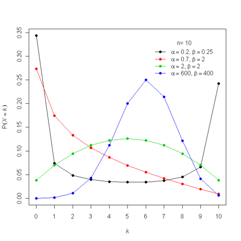
This distribution is called the beta-binomial distribution. Below is an image from Wikipedia showing a graph of \(p(X)\) for \(N=10\) and a number of different values of \(a\) and \(b\). You can see that, especially for small value of \(a\) and \(b\) the distribution is a lot more spread out than the binomial distribution. This is because there is randomness coming from both \(\rho\) and the binomial conditional distribution.