One of the great results of the 19th century German mathematician Georg Cantor is that the sets \(\mathbb{N}\) and \(\mathbb{N} \times \mathbb{N}\) have the same cardinality. That is the set of all non-negative integers \(\mathbb{N} = \{0,1,2,3,\ldots\}\) has the same size as the set of all pairs on non-negative integers \(\mathbb{N} \times \mathbb{N} = \{(m,n) \mid m,n \in \mathbb{N} \}\), or put less precisely “infinity times infinity equals infinity”.
Proving this result amounts to finding a bijection \(p : \mathbb{N} \times \mathbb{N} \to \mathbb{N}\). We will call such a function a pairing function since it takes in two numbers and pairs them together to create a single number. An example of one such function is
\(p(m,n) = 2^m(2n+1)-1\)
This function is a bijection because every positive whole number can be written uniquely as the product of a power of two and an odd number. Such functions are of practical as well as theoretical interest. Computers use pairing functions to store matrices and higher dimensional arrays. The entries of the matrix are actually stored in a list. When the user gives two numbers corresponding to a matrix entry, the computer uses a pairing function to get just one number which gives the index of the corresponding entry in the list. Thus having efficiently computable pairing functions is of practical importance.
Representing Pairing Functions
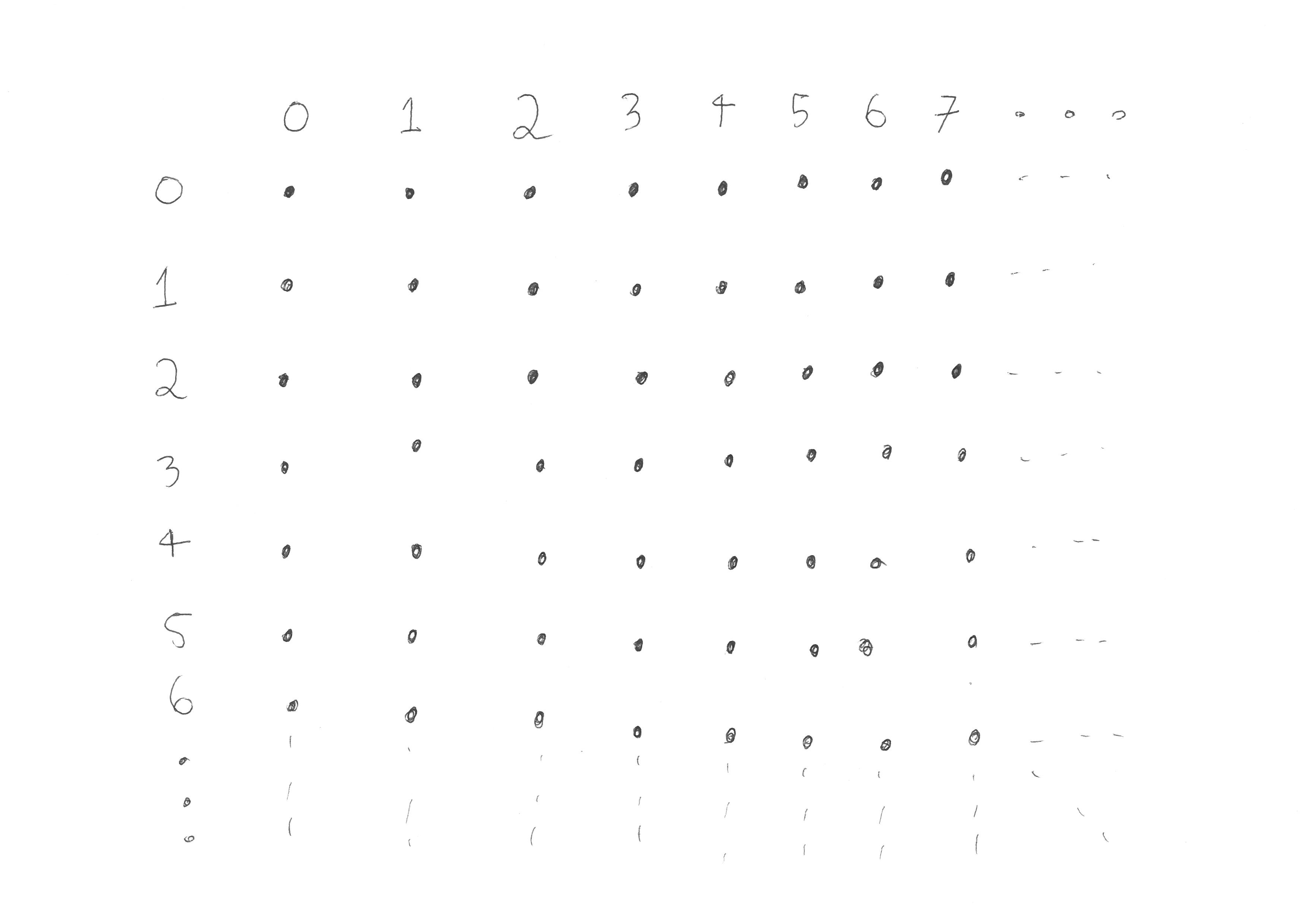
Our previous example of a pairing function was given by a formula. Another way to define pairing functions is by first representing the set \(\mathbb{N} \times \mathbb{N}\) as a grid with an infinite number of rows and columns like so:
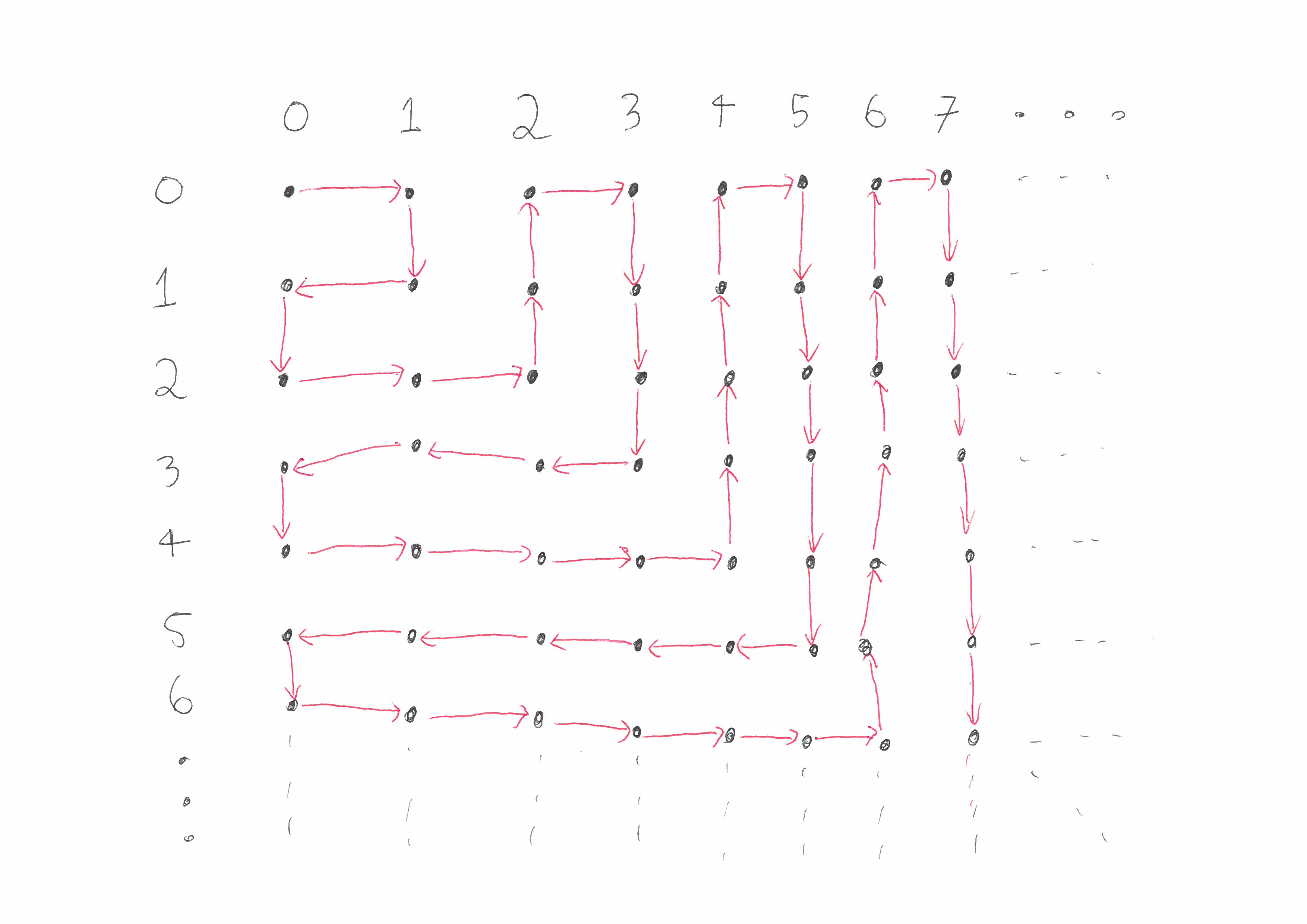
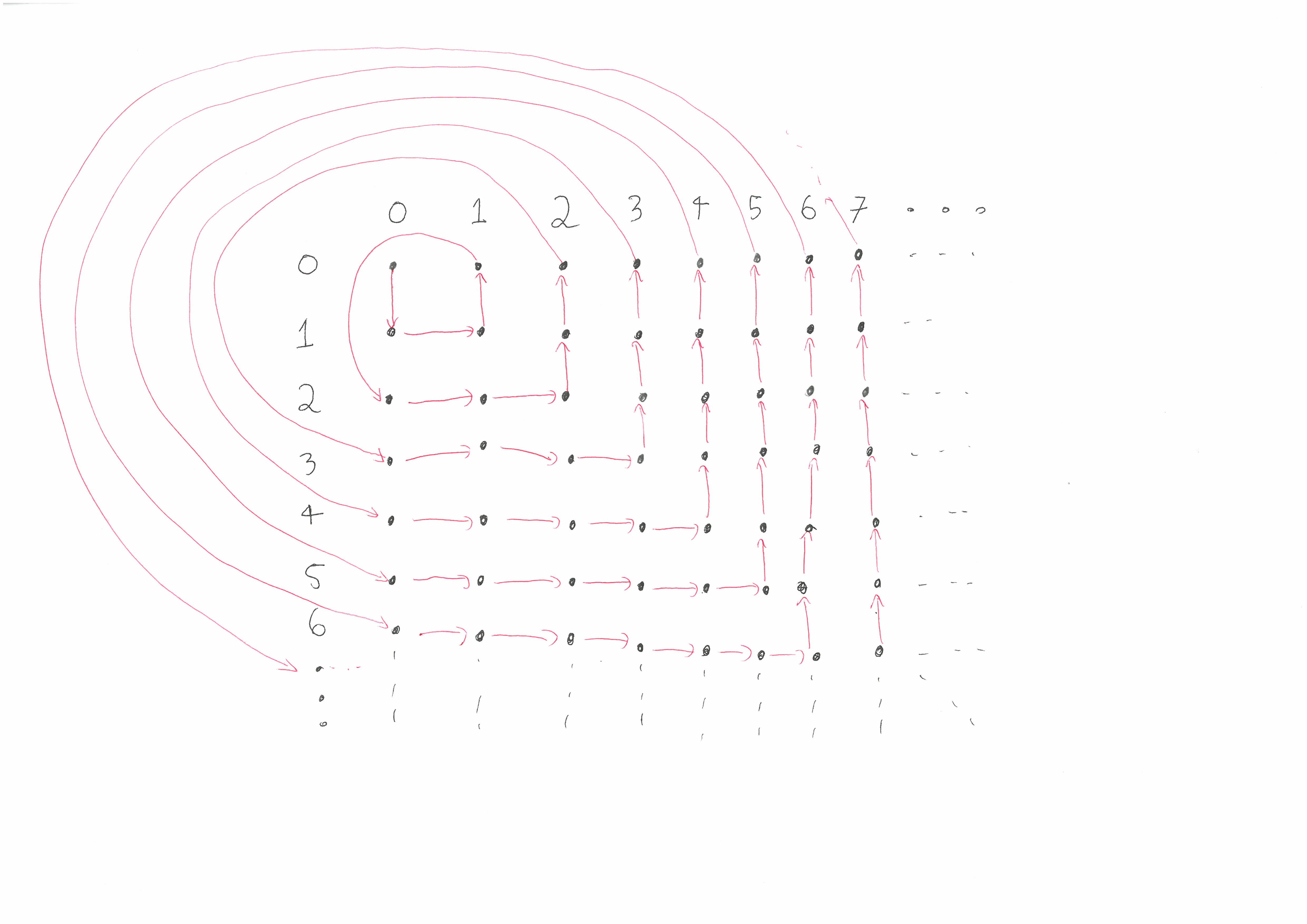
We can then represent a pairing function as a path through this grid that passes through each square exactly once. Here are two examples:
The way to go from one of these paths to a function from \(\mathbb{N} \times \mathbb{N}\) to \(\mathbb{N}\) is as follows. Given as input a pair of integers \((m,n)\), first find the dot that \((m,n)\) represents in the grid. Next count the number of backwards steps that need to be taken to get to the start of the path and then output this number.
We can also do the reverse of the above procedure. That is, given a pairing function \(p : \mathbb{N} \times \mathbb{N} \to \mathbb{N}\), we can represent \(p\) as a path in the grid. This is done by starting at \(p^{-1}(0)\) and joining \(p^{-1}(n)\) to \(p^{-1}(n+1)\). It’s a fun exercise to work out what the path corresponding to \(p(m,n) = 2^m(2n+1)-1\) looks like.
Cantor’s Pairing Function
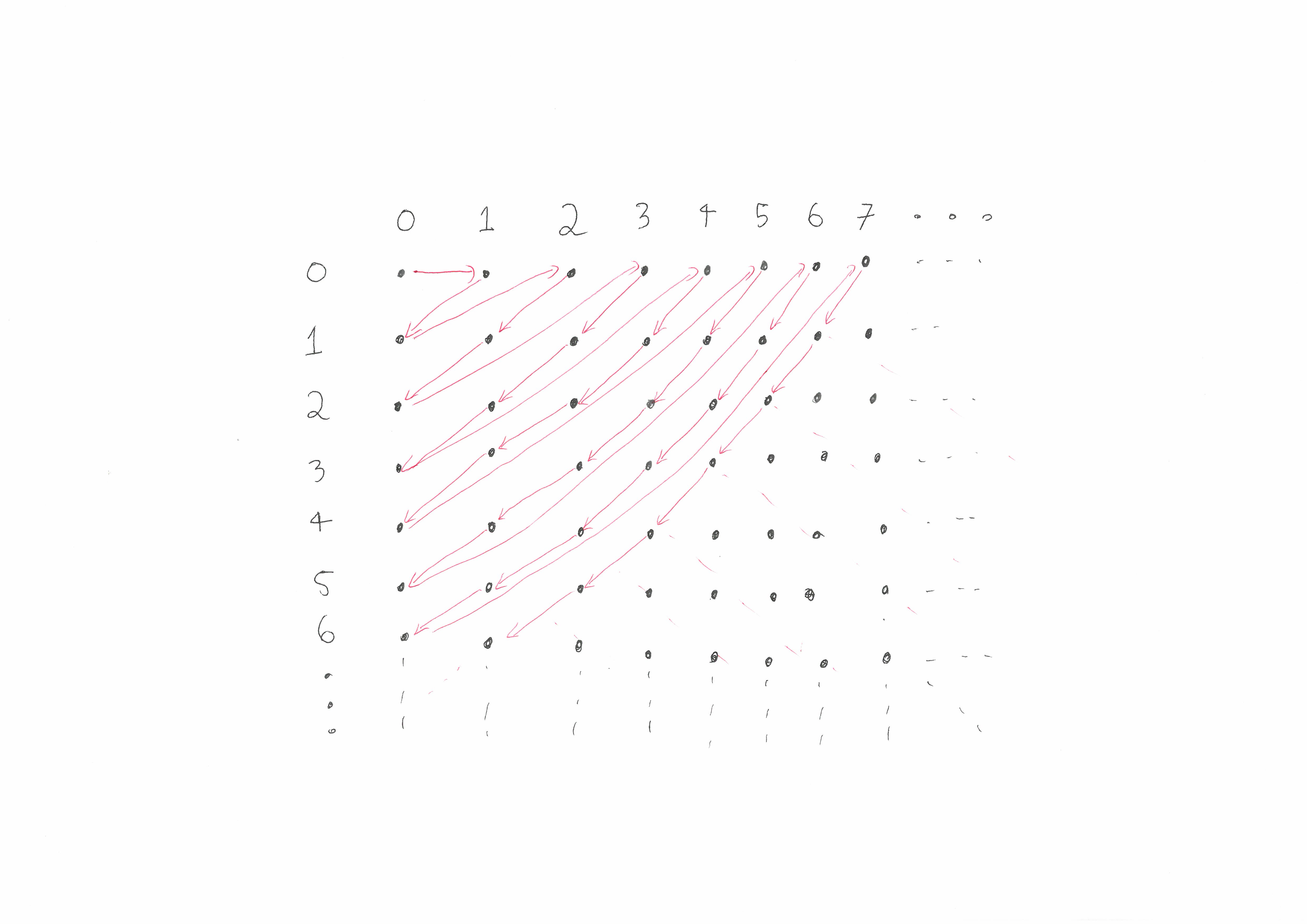
The pairing function that Cantor used is not any of the ones we have seen so far. Cantor used a pairing function which we will call \(q\). When represented as a path, this is what \(q\) looks like:
Surprisingly there’s a simple formula that represents this pairing function \(q\) which we will now derive. First note that if we are at a point \((k,0)\), then the value of \(q(k,0)\) is \(1+2+3+\ldots+(k-1)+k= \frac{1}{2}k(k+1)\). This is because to get to \((k,0)\) from \((0,0) = q^{-1}(0)\), we have to go along \(k\) diagonals which each increase in length.
Now let \((m,n)\) be an arbitrary pair of integers and let \(k = m+n\). The above path first goes through \((k,0)\) and then takes \(n\) steps to get to \((m,n)\). Thus
And so Cantor’s pairing function is actually a quadratic polynomial in two variables!
Other Polynomial Pairing Functions?
Whenever we have a pairing function \(p\), we can switch the order of the inputs and get a new pairing function \(\widetilde{p}\). That is the function \(\widetilde{p}\) is given by \(\widetilde{p}(m,n)=p(n,m)\). When thinking of pairing functions as paths in a grid, this transformation amounts to reflecting the picture along the diagonal \(m = n\).
Cantor’s function q
The switched version of q
Thus there are at least two quadratic pairing functions, Cantor’s function \(q\) and its switched cousin \(\widetilde{q}\). The Fueter–Pólya theorem states these two are actually the only quadratic pairing functions! In fact it is conjectured that these two quadratics are the only polynomial pairing functions but this is still an open question.
Thank you to Wikipedia!
I first learnt that the sets \(\mathbb{N}\) and \(\mathbb{N} \times \mathbb{N}\) have the same cardinality in class a number of years ago. I only recently learnt about Cantor’s polynomial pairing function and the Fueter–Pólya theorem by stumbling across the Wikipedia page for pairing functions. Wikipedia is a great source for discovering new mathematics and for checking results. I use Wikipedia all the time. Many of these blog posts were initially inspired by Wikipedia entries.
Currently, Wikipedia is doing their annual fundraiser. If you are a frequent user of Wikipedia like me, I’d encourage you to join me in donating a couple of dollars to them: https://donate.wikimedia.org.
Last semester I tutored the course Probability Modelling with Applications. In this course the main objects of study are probability spaces. A probability space is a triple \((\Omega, \mathcal{F}, \mathbb{P})\) where:
\(\Omega\) is a set.
\(\mathcal{F}\) is a \(\sigma\)-algebra on \(\Omega\). That is \(\mathcal{F}\) is a collection of subsets of \(\Omega\) such that \(\Omega \in \mathcal{F}\) and \(\mathcal{F}\) is closed under set complements and countable unions. The element of \(\mathcal{F}\) are called events and they are precisely the subsets of \(\Omega\) that we can assign probabilities to. We will denote the power set of \(\Omega\) by \(2^\Omega\) and hence \(\mathcal{F} \subseteq 2^\Omega\).
\(\mathbb{P}\) is a probability measure. That is it is a function \(\mathbb{P}: \mathcal{F} \rightarrow [0,1]\) such that \(\mathbb{P}(\Omega)=1\) and for all countable collections \(\{A_i\}_{i=1}^\infty \subseteq \mathcal{F}\) of mutually disjoint subsets we have that \(\mathbb{P} \left(\bigcup_{i=1}^\infty A_i \right) = \sum_{i=1}^\infty \mathbb{P}(A_i) \).
It’s common for students to find probability spaces, and in particular \(\sigma\)-algebras, confusing. Unfortunately Vitalli showed that \(\sigma\)-algebras can’t be avoided if we want to study probability spaces such as \(\mathbb{R}\) or an infinite number of coin tosses. One of the main reasons why \(\sigma\)-algebras can be so confusing is that it can be very hard to give concrete descriptions of all the elements of a \(\sigma\)-algebra.
We often have a collection \(\mathcal{G}\) of subsets of \(\Omega\) that we are interested in but this collection fails to be a \(\sigma\)-algebra. For example, we might have \(\Omega = \mathbb{R}^n\) and \(\mathcal{G}\) is the collection of open subsets. In this situation we take our \(\sigma\)-algebra \(\mathcal{F}\) to be \(\sigma(\mathcal{G})\) which is the smallest \(\sigma\)-algebra containing \(\mathcal{G}\). That is
\(\sigma(\mathcal{G}) = \bigcap \mathcal{F}’\)
where the above intersection is taken over all \(\sigma\)-algebras \(\mathcal{F}’\) that contain \(\mathcal{G}\). In this setting we will say that \(\mathcal{G}\) generates \(\sigma(\mathcal{G})\). When we have such a collection of generators, we might have an idea for what probability we would like to assign to sets in \(\mathcal{G}\). That is we have a function \(\mathbb{P}_0 : \mathcal{G} \rightarrow [0,1]\) and we want to extend this function to create a probability measure \(\mathbb{P} : \sigma(\mathcal{G}) \rightarrow [0,1]\). A famous theorem due to Caratheodory shows that we can do this in many cases.
An interesting question is whether the extension \(\mathbb{P}\) is unique. That is does there exists a probability measure \(\mathbb{P}’\) on \(\sigma(\mathcal{G})\) such that \(\mathbb{P} \neq \mathbb{P}’\) but \(\mathbb{P}_{\mid \mathcal{G}} = \mathbb{P}_{\mid \mathcal{G}}’\)? The following theorem gives a criterion that guarantees no such \(\mathbb{P}’\) exists.
Theorem: Let \(\Omega\) be a set and let \(\mathcal{G}\) be a collection of subsets of \(\Omega\) that is closed under finite intersections. Then if \(\mathbb{P},\mathbb{P}’ : \sigma(\mathcal{G}) \rightarrow [0,1]\) are two probability measures such that \(\mathbb{P}_{\mid \mathcal{G}} = \mathbb{P}’_{\mid \mathcal{G}}\), then \(\mathbb{P} = \mathbb{P}’\).
The above theorem is very useful for two reasons. Firstly it can be combined with Caratheodory’s extension theorem to uniquely define probability measures on a \(\sigma\)-algebra by specifying the values on a collection of simple subsets \(\mathcal{G}\). Secondly if we ever want to show that two probability measures are equal, the above theorem tells us we can reduce the problem to checking equality on the simpler subsets in \(\mathcal{G}\).
The condition that \(\mathcal{G}\) must be closed under finite intersections is somewhat intuitive. Suppose we had \(A,B \in \mathcal{G}\) but \(A \cap B \notin \mathcal{G}\). We will however have \(A \cap B \in \sigma(\mathcal{G})\) and thus we might be able to find two probability measure \(\mathbb{P},\mathbb{P}’ : \sigma(\mathcal{G}) \rightarrow [0,1]\) such that \(\mathbb{P}(A) = \mathbb{P}'(A)\) and \(\mathbb{P}'(B)=\mathbb{P}'(B)\) but \(\mathbb{P}(A \cap B) \neq \mathbb{P}'(A \cap B)\). The following counterexample shows that this intuition is indeed well-founded.
When looking for examples and counterexamples, it’s good to try to keep things as simple as possible. With that in mind we will try to find a counterexample when \(\Omega\) is finite set with as few elements as possible and \(\sigma(\mathcal{G})\) is equal to the powerset of \(\Omega\). In this setting, a probability measure \(\mathbb{P}: \sigma(\mathcal{G}) \rightarrow [0,1]\) can be defined by specifying the values \(\mathbb{P}(\{\omega\})\) for each \(\omega \in \Omega\).
We will now try to find a counterexample when \(\Omega\) is as small as possible. Unfortunately we won’t be able find a counterexample when \(\Omega\) only contains one or two elements. This is because we want to find \(A,B \subseteq \Omega\) such that \(A \cap B\) is not equal to \(A,B\) or \(\emptyset\).
Thus we will start out search with a three element set \(\Omega = \{a,b,c\}\). Up to relabelling the elements of \(\Omega\), the only interesting choice we have for \(\mathcal{G}\) is \(\{ \{a,b\} , \{b,c\} \}\). This has a chance of working since \(\mathcal{G}\) is not closed under intersection. However any probability measure \(\mathbb{P}\) on \(\sigma(\mathcal{G}) = 2^{\{a,b,c\}}\) must satisfy the equations
Thus \(\mathbb{P}(\{a\}) = 1- \mathbb{P}(\{b,c\})\), \(\mathbb{P}(\{c\}) = 1-\mathbb{P}(\{a,b\})\) and \(\mathbb{P}(\{b\})=\mathbb{P}(\{a,b\})+\mathbb{P}(\{b,c\})-1\). Thus \(\mathbb{P}\) is determined by its values on \(\{a,b\}\) and \(\{b,c\}\).
However, a four element set \(\{a,b,c,d\}\) is sufficient for our counter example! We can let \(\mathcal{G} = \{\{a,b\},\{b,c\}\}\). Then \(\sigma(\mathcal{G})=2^{\{a,b,c,d\}}\) and we can define \(\mathbb{P} , \mathbb{P}’ : \sigma (\mathcal{G}) \rightarrow [0,1]\) by
\(\mathbb{P}(\{a\}) = 0\), \(\mathbb{P}(\{b\})=0.5\), \(\mathbb{P}(\{c\})=0\) and \(\mathbb{P}(\{d\})=0.5\).
\(\mathbb{P}'(\{a\})=0.5\), \(\mathbb{P}(\{b\})=0\), \(\mathbb{P}(\{c\})=0.5\) and \(\mathbb{P}(\{d\})=0\).
Clearly \(\mathbb{P} \neq \mathbb{P}’\) however \(\mathbb{P}(\{a,b\})=\mathbb{P}'(\{a,b\})=0.5\) and \(\mathbb{P}(\{b,c\})=\mathbb{P}'(\{b,c\})=0.5\). Thus we have our counterexample! In general for any \(\lambda \in [0,1)\) we can define the probability measure \(\mathbb{P}_\lambda = \lambda\mathbb{P}+(1-\lambda)\mathbb{P}’\). The measure \(\mathbb{P}_\lambda\) is not equal to \(\mathbb{P}\) but agrees with \(\mathbb{P}\) on \(\mathcal{G}\). In general, if we have two probability measures that agree on \(\mathcal{G}\) but not on \(\sigma(\mathcal{G})\) then we can produce uncountably many such measures by taking convex combinations as done above.
Earlier in the year I wrote a post on Less Wrong about some of the material I learnt at the 2019 AMSI Summer School. You can read it here. On a related note, applications are open for the 2020 AMSI Summer School at La Trobe University. I highly recommend attending!
Two weeks ago I gave talk titled “Two Combings of \(\mathbb{Z}^2\)”. The talk was about some material I have been discussing lately with my honours supervisor. The talk went well and I thought it would be worth sharing a written version of what I said.
Geometric Group Theory
Combings are a tool that gets used in a branch of mathematics called geometric group theory. Geometric group theory is a relatively new area of mathematics and is only around 30 years old. The main idea behind geometric group theory is to use tools and ideas from geometry and low dimensional topology to study and understand groups. It turns out that some of the simplest questions one can ask about groups have interesting geometric answers. For instance, the Dehn function of a group gives a natural geometric answer to the solvability of the word problem.
Generators
Before we can define what a combing is we’ll need to set up some notation. If \(A\) is a set then we will write \(A^*\) for the set of words written using elements of \(A\) and inverses of elements of \(A\). For instance if \(A = \{a,b\}\), then \(A^* = \{\varepsilon, a,b,a^{-1},b^{-1},aa=a^2,abb^{-1}a^{-3},\ldots\}\) (here \(\varepsilon\) refers to the empty word). If \(w\) is a word in \(A^*\), we will write \(l(w)\) for the length of \(w\). Thus \(l(\varepsilon)=0, l(a)=1, l(abb^{-1}a^{-3})=6\) and so on.
If \(G\) is a group and \(A\) is a subset of \(G\), then we have a natural map \(\pi : A^* \rightarrow G\) given by:
We will say that \(A\) generates \(G\) if the above map is surjective. In this case we will write \(\overline{w}\) for \(\pi(w)\) when \(w\) is a word in \(A^*\).
The Word Metric
The geometry in “geometric group theory” often arises when studying how a group acts on different geometric spaces. A group always acts on itself by left multiplication. The following definition adds a geometric aspect to this action. If \(G\) is a group with generators \(A\), then the word metric on \(G\) with respect to \(A\) is the function \(d_G : G \times G \rightarrow \mathbb{R}\) given by
That, is the distance between two group elements \(g,h \in G\) is the length of the shortest word in \(A^*\) we can use to represent \(g^{-1}h\). Equivalently the distance between \(g\) and \(h\) is the length of the shortest word we have to append to \(g\) to produce \(h\). This metric is invariant under left-multiplication by \(G\) (ie \(d_G(g\cdot h,g\cdot h’) =d_G(h,h’)\) for all \(g,h,h’ \in G\)). Thus \(G\) acts on \((G,d_G)\) by isometries.
Words are Paths
Now that we are viewing the group \(G\) as a geometric space, we can also change how we think of words \(w \in A^*\). Such a word can be thought of as discrete path in \(G\). That is we can think of \(w\) as a function from \(\mathbb{N}\) to \(G\). This way of thinking of \(w\) as a discrete path is best illuminated with an example. Suppose we have the word \(w = ab^2a^{-1}b\), then
Thus the path \(w : \mathbb{N} \rightarrow G\) is given by taking the first \(t\) letters of \(w\) and mapping this word to the group element it represents. With this interpretation of word in \(A^*\) in mind we can now define combings.
Combings
Let \(G\) be a group with a finite set of generators \(A\). Then a combing of \(G\) with respect to \(A\) is a function \(\sigma : G \rightarrow A^*\) such that
For all \(g \in G\), \(\overline{\sigma_g} = g\) (we will write \(\sigma_g\) for \(\sigma(g))\).
There exists \(k >0\) such that for all \( g, h \in G\) with \(g \cdot \overline{a} = h\) for some \(a \in A\), we have that \(d_G(\sigma_g(t),\sigma_h(t)) \le k\) for all \(t \in \mathbb{N}\).
The first condition says that we can think of \(\sigma\) as a way of picking a normal form \(\sigma_g \in A^*\) for each \(g \in G\). The second condition is a bit more involved. It states that if the group elements \(g, h \in G\) are distance 1 from each other in the word metric, then the paths \(\sigma_g,\sigma_h : \mathbb{N} \rightarrow G\) are within distance \(k\) of each other at any point in time.
An Example
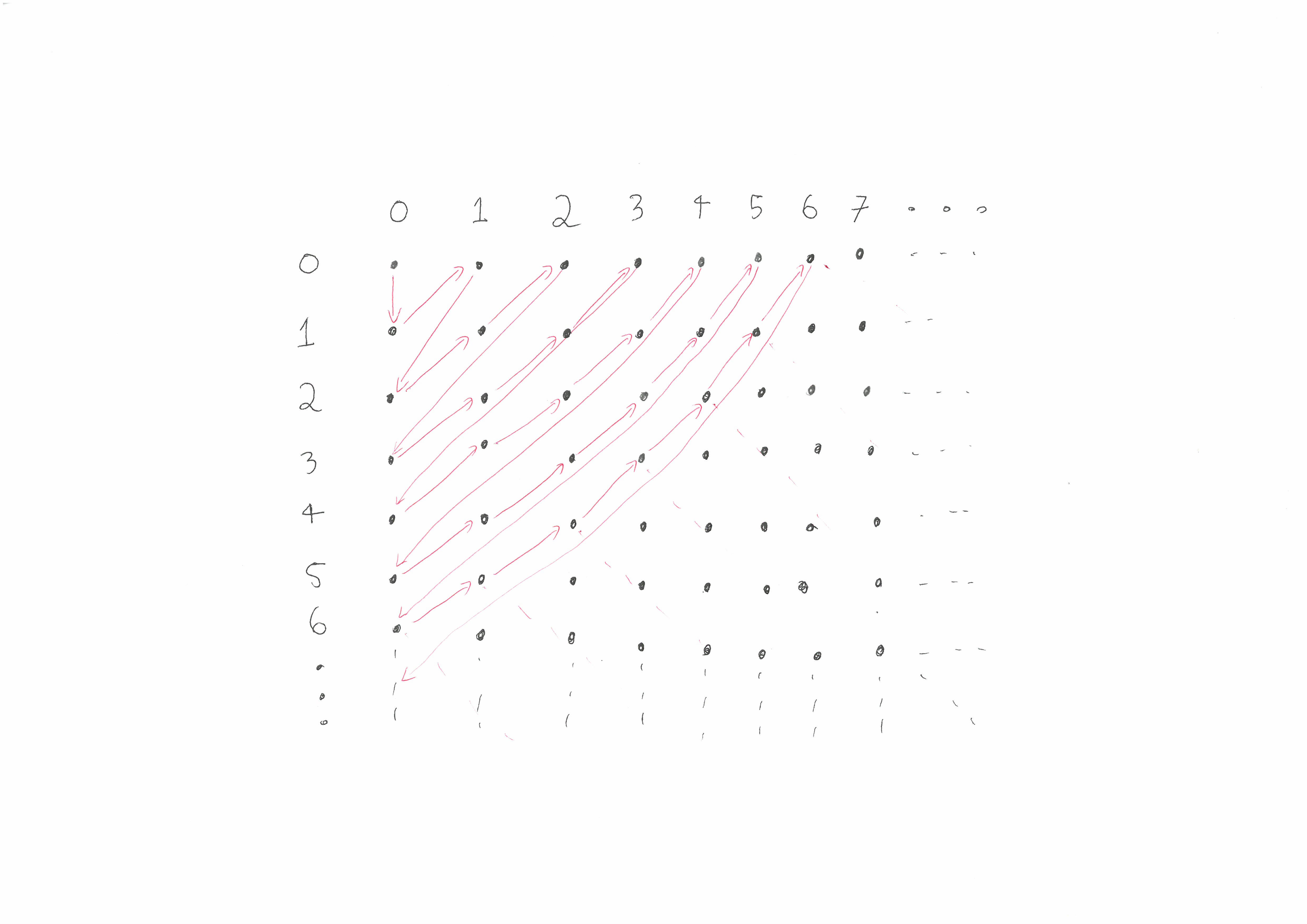
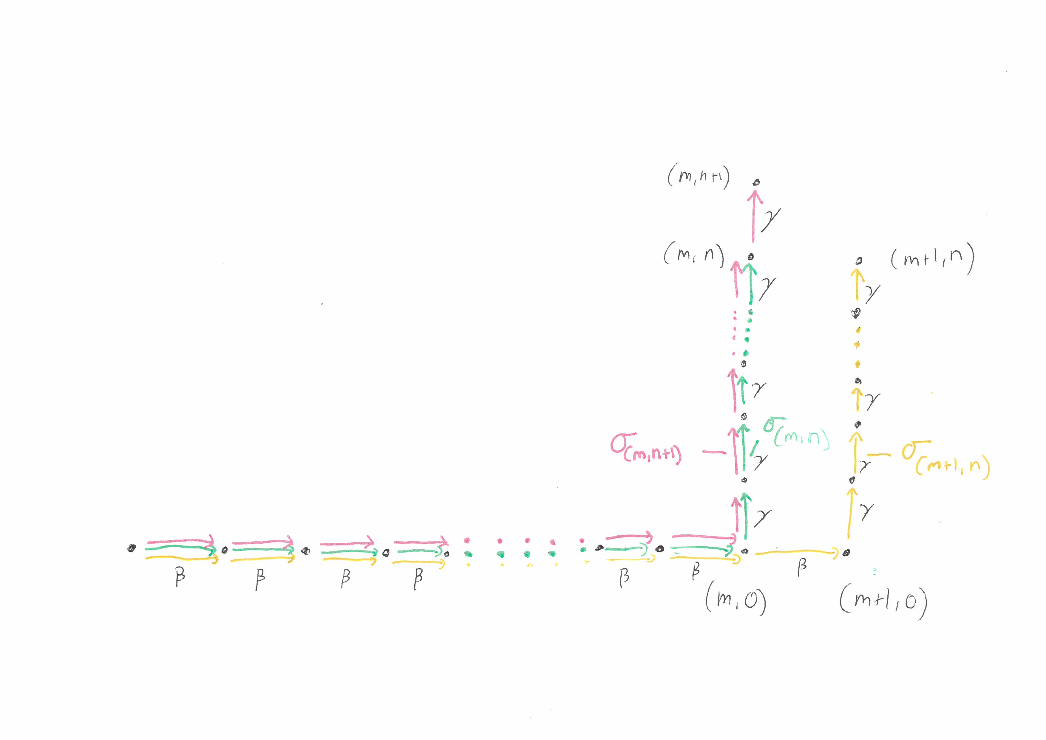
Not all groups can be given a combing. Indeed if we have a combing of \(G\), then the word problem in \(G\) is solvable and the Dehn function of \(G\) is at most exponential. One group that does admit a combing is \(\mathbb{Z}^2 = \{(m,n) \mid m,n \in \mathbb{Z}\}\). This group is generated by \(A = \{(1,0),(0,1)\} = \{\beta,\gamma\}\) and one combing of \(\mathbb{Z}^2\) with respect to this generating set is
\(\sigma_{(m,n)} = \beta^m\gamma^n\).
The first condition of being a combing is clearly satisfied and the following picture shows that the second condition can be satisfied with \(k = 2\).
That is, the group \(H_3\) has three generators \(\alpha,\beta\) and \(\gamma\). The generator \(\gamma\) commutes with both \(\alpha\) and \(\beta\). The generators \(\alpha\) and \(\beta\) almost commute but don’t quite as seen in the relation \(\beta\alpha = \alpha\beta\gamma\).
Any \(h \in H_3\) can be represented uniquely as \(\sigma_h = \alpha^p\beta^m\gamma^n\) for \(p,m,n \in \mathbb{Z}\). To see why such a representation exists it’s best to consider an example. Suppose that \(h = \overline{\gamma\beta\alpha\gamma\alpha\beta\gamma}\). Then we can use the fact that \(\gamma\) commutes with \(\alpha\) and \(\beta\) to push all \(\gamma\)’s to the right and we get that \(h = \overline{\beta\alpha\alpha\beta\gamma^3}\). We can then apply the third relation to switch the order of \(\alpha\) and \(\beta\) on the right. This gives us that that \(h = \overline{\alpha\beta\gamma\alpha\beta\gamma^3}=\overline{\alpha\beta\alpha\beta\gamma^4}\). If we apply this relation once more we get that \(h = \overline{\alpha^2\beta^2\gamma^5}\) and thus \(\sigma_h = \alpha^2\beta^2\gamma^5\). The procedure used to write \(h\) in the form \(\alpha^p\beta^m\gamma^n\) can be generalized to any word written using \(\alpha^{\pm 1}, \beta^{\pm 1}, \gamma^{\pm 1}\).
The fact the such a representation is unique (that is if \(\overline{\alpha^p\beta^m\gamma^n} = \overline{\alpha^{p’}\beta^{m’}\gamma^{n’}}\), then \((p,m,n) = (p’,m’,n’)\)) is harder to justify but can be proved by defining an action of \(H_3\) on \(\mathbb{Z}^3\). Thus we can define a function \(\sigma : H_3 \rightarrow \{\alpha,\beta,\gamma\}^*\) by setting \(\sigma_h\) to be the unique word of the form \(\alpha^p \beta^m\gamma^n\) that represents \(h\). This map satisfies the first condition of being a combing and has many nice properties. These include that it is easy to check whether or not a word in \(\{\alpha,\beta,\gamma\}^*\) is equal to \(\sigma_h\) for some \(h \in H_3\) and there are fast algorithms for putting a word in \(\{\alpha,\beta,\gamma\}^*\) into its normal form. Unfortunately this map fails to be a combing.
The reason why \(\sigma : H_3 \rightarrow \{\alpha,\beta,\gamma\}^*\) fails to be a combing can be seen back when we turned \(\overline{ \gamma\beta\alpha\gamma\alpha\beta\gamma }\) into \( \overline{\alpha^2\beta^2\gamma^5} \). To move \(\alpha\)’s on the right to the left we had to move past \(\beta\)’s and produce \(\gamma\)’s in the process. More concretely fix \(m \in \mathbb{N}\) and let \(h = \overline{\beta^m}\) and \(g = \overline{\beta^m \alpha} = \overline{\alpha \beta^m\gamma^m}\). We have \(\sigma_h = \beta^m\) and \(\sigma_g = \alpha \beta^m \gamma^m\). The group elements \(g\) and \(h\) differ by a generator. Thus, if \(\sigma\) was a combing we should be able to uniformly bound \(d_{H_3}(\sigma_g(t),\sigma_h(t))\) for all \(t \in \mathbb{N}\) and all \(m \in \mathbb{N}\).
If we then let \(t = m+1\), we can recall that
\(d_{H_3}(\sigma_g(t),\sigma_h(t)) = \min\{l(w) \mid w \in \{\alpha,\beta,\gamma\}^*, \overline{w} = \sigma_g(t)^{-1}\sigma_h(t)\}.\)
We have that \(\sigma_h(t) = \overline{\beta^m}\) and \(\sigma_g(t) = \overline{\alpha \beta^m}\) and thus
The group element \(\overline{\alpha^{-1}\gamma^{m}}\) cannot be represented as a shorter element of \(\{\alpha,\beta,\gamma\}^*\) and thus \(d_{H_3}(\sigma_g(t),\sigma_h(t)) = m+1\) and the map \(\sigma \) is not a combing.
Can we comb the Heisenberg group?
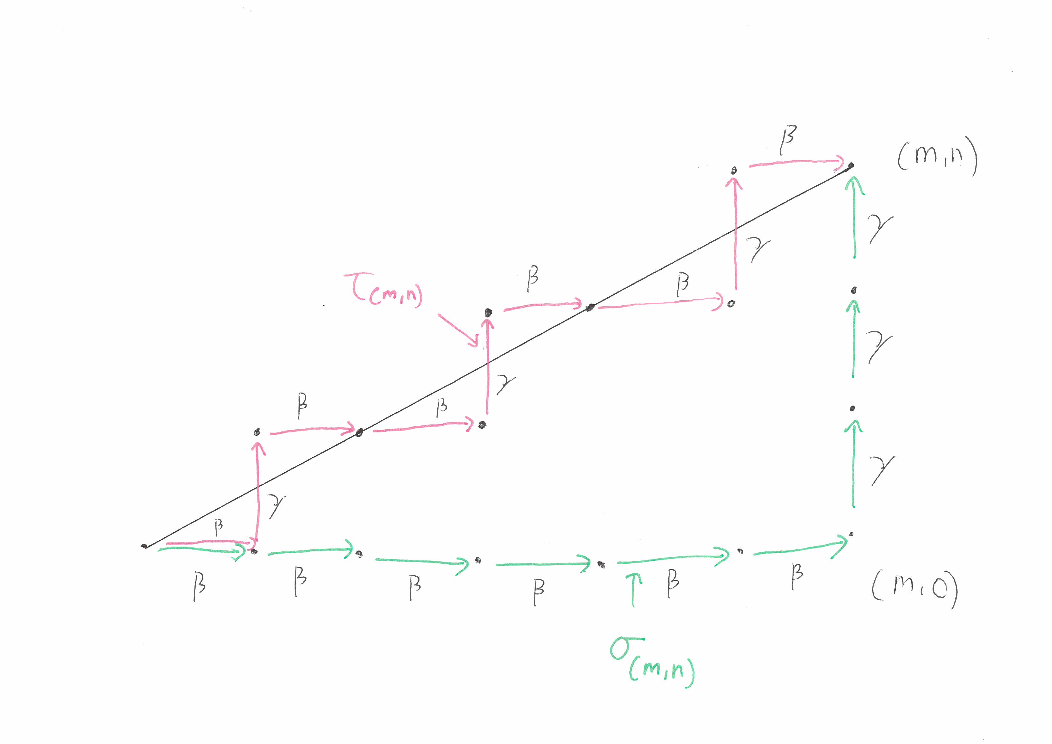
This leaves us with a question, can we comb the group \(H_3\)? It turns out that we can but the answer actually lies in finding a better combing of \(\mathbb{Z}^2\). This is because \(H_3\) contains the subgroup \(\mathbb{Z}^2 \cong \langle \beta, \gamma \rangle \subseteq H_3\). Rather than using the normal form \(\sigma_h = \alpha^p \beta^m \gamma^n\), we will use \(\sigma’_h = \alpha^p \tau_{(m,n)}\) where \(\tau : \mathbb{Z}^2 \rightarrow \{\beta,\gamma \}^*\) is a combing of \(\mathbb{Z}^2\) that is more symmetric. The word \(\tau_{(m,n)}\) is defined to be the sequence of \(m \) \(\beta\)’s and \(n\) \(\gamma\)’s that stays closest to the straight line in \(\mathbb{R}^2\) that joins \((0,0)\) to \((n,p)\) (when we view \(\beta\) and \(\gamma\) as representing \((1,0)\) and \((0,1)\) respectively). Below is an illustration:
This new function isn’t quite a combing of \(H_3\) but it is the next best thing! It is anasynchronous combing. An asynchronous combing is one where we again require that the paths \(\sigma_h,\sigma_g\) stay close to each other whenever \(h\) and \(g\) are close to each other. However we allow the paths \(\sigma_h\) and \(\sigma_g\) to travel at different speeds. Many of the results that can be proved for combable groups extend to asynchronously combable groups.
References
Hairdressing in Groups by Sarah Rees is a survey paper that includes lots examples of groups that do or do not admit combings. It also talks about the language complexity of a combing, something I didn’t have time to touch on in my talk.
Combings of Semidirect Products and 3-Manifold Groups by Martin Bridson contains a proof that \(H_3\) is asynchornously combable. He actually proves the more general result that any group of the form \(\mathbb{Z}^n \rtimes \mathbb{Z}^m\) is asynchronously combable.
Thank you to my supervisor, Tony Licata, for suggesting I give my talk on combing \(H_3\) and for all the support he has given me so far.