Tag: mathematics

  • Total Variation and Marathon Running

    Total variation is a way of measuring how much a function \(f:[a,b] \to \mathbb{R}\) “wiggles”. In this post, I want to motivate the definition of total variation by talking about elevation in marathon running.

    Comparing marathon courses

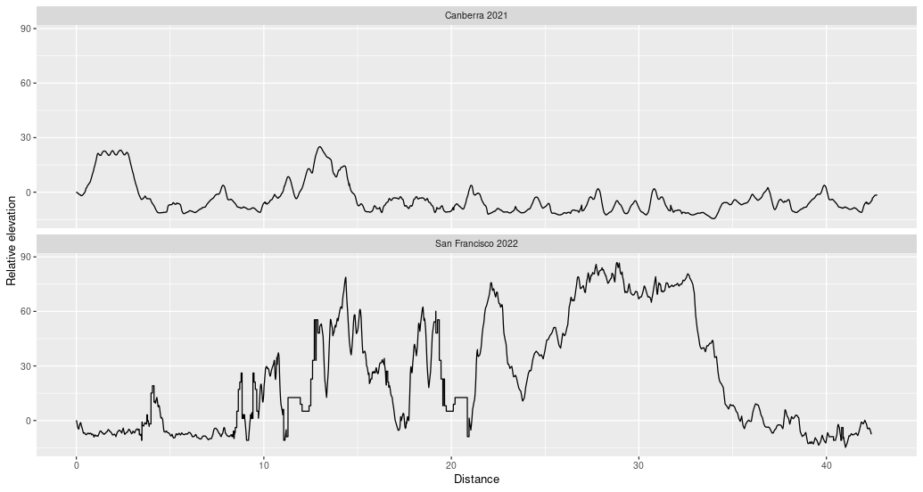
    On July 24th I ran the 2022 San Francisco (SF) marathon. All marathons are the same distance, 42.2 kilometres (26.2 miles) but individual courses can vary greatly. Some marathons are on road and others are on trails. Some locations can be hot and others can be rainy. And some, such as the SF marathon, can be much hillier than others. Below is a plot comparing the elevation of the Canberra marathon I ran last year to the elevation of the SF marathon:

    A plot showing the relative elevation over the course of the Canberra and San Francisco marathons. Try to spot the two times I ran over the Golden Gate Bridge during the SF marathon.

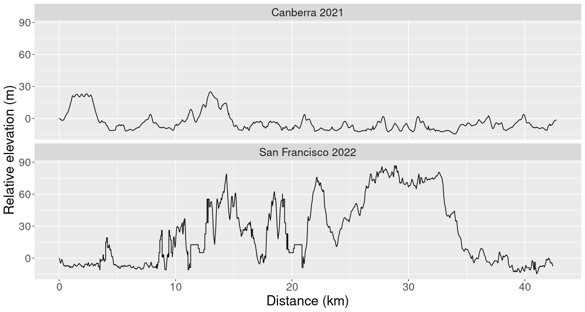
    Immediately, you can see that the range of elevation during the San Francisco marathon was much higher than the range of elevation during the Canberra marathon. However, what made the SF marathon hard wasn’t any individual incline but rather the sheer number of ups and downs. For comparison, the plot below shows elevation during a 32 km training run and elevation during the SF marathon:

    A plot showing the relative elevation over the course of a training run and the San Francisco marathon. The big climb during my training run is the Stanford dish.

    You can see that my training run was mostly flat but had one big hill in the last 10 kilometres. The maximum relative elevation on my training run was about 50 meters higher than the maximum relative elevation of the marathon, but overall the training run graph is a lot less wiggly. This meant there were far more individual hills during the marathon and so the first 32 km of the marathon felt a lot tougher than the training run. By comparing these two runs, you can see that the elevation range can hide important information about the difficulty of a run. We also need to pay attention to how wiggly the elevation curve is.

    Wiggliness Scores

    So far our definition of wiggliness has been imprecise and has relied on looking at a graph of the elevation. This makes it hard to compare two runs and quickly decide which one is wigglier. It would be convenient if there was a “wiggliness score” – a single number we could assign to each run which measured the wiggliness of the run’s elevation. Bellow we’ll see that total variation does exactly this.

    If we zoom in on one of the graphs above, we would see that it actually consists of tiny straight line segments. For example, let’s look at the 22nd kilometre of the SF marathon. In this plot it looks like elevation is a smooth function of distance:

    The relative elevation of the 22nd kilometre during the SF marathon.

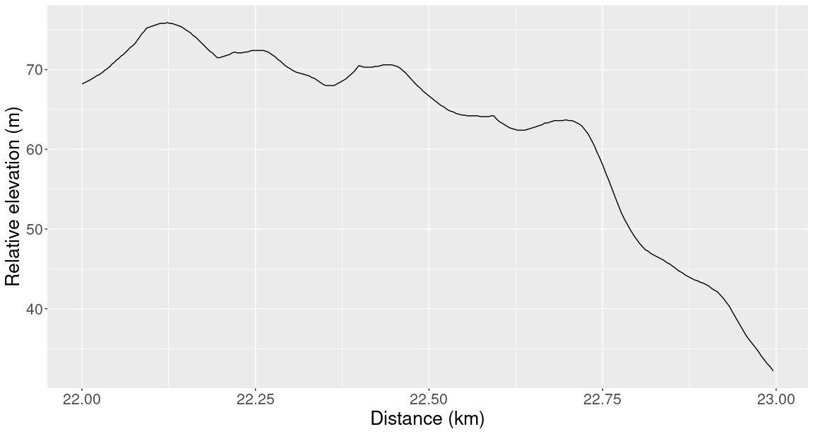
    But if we zoom in on a 100 m stretch, then we see that the graph is actually a series of straight lines glued together:

    The relative elevation over a 100 metres during the marathon.

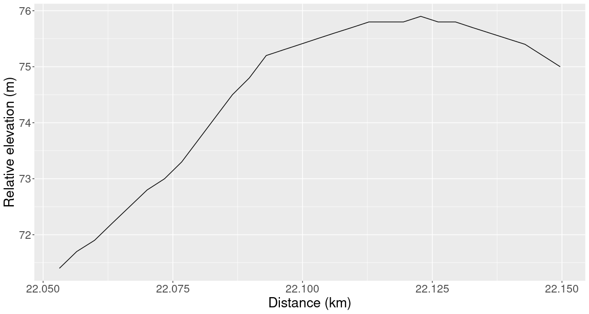
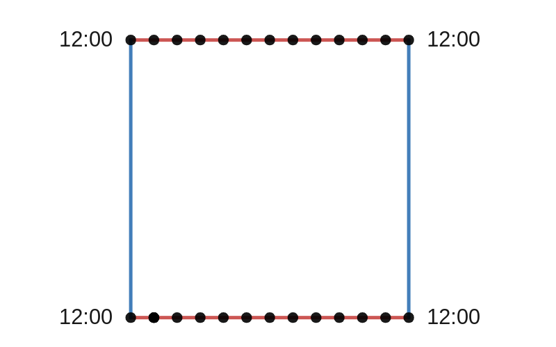
    This is because these graphs are made using my GPS watch which makes one recording per second. If we place dots at each of these times, then the straight lines become clearer:

    The relative elevation over the same 100 metre stretch. Each blue dots marks a point when a measurement was made.

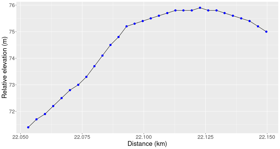
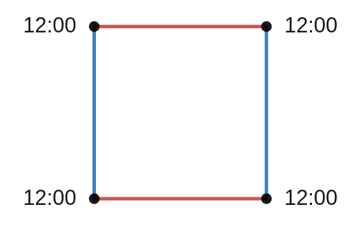
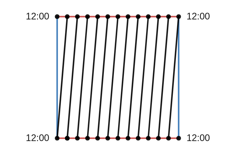
    We can use these blue dots to define the graph’s wiggliness score. The wiggliness score should capture how much the graph varies across its domain. This suggests that wiggliness scores should be additive. By additive, I mean that if we split the domain into a finite number of pieces, then the wiggliness score across the whole domain should be the sum of the wiggliness score of each segment.

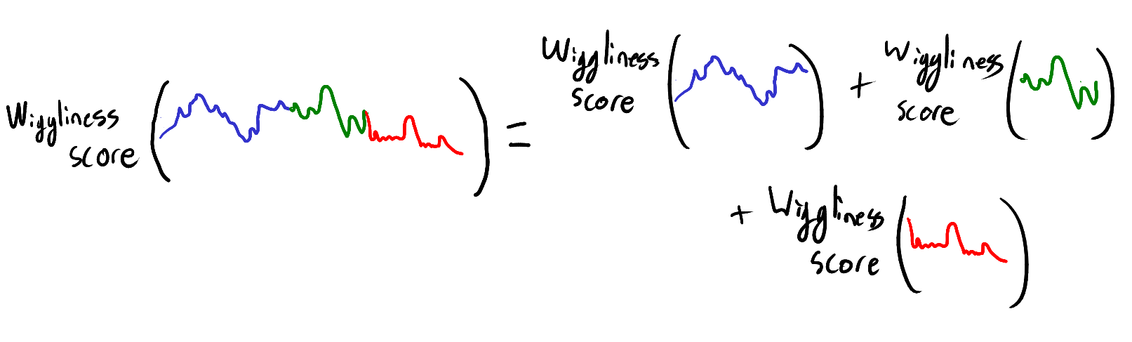
    In particular, the wiggliness score for the SF marathon is equal to the sum of the wiggliness score of each section between two consecutive blue dots. This means we only need to quantify how much the graph varies between consecutive blue dots. Fortunately, between two such dots, the graph is a straight line. The amount that a straight line varies is simply the distance between the y-value at the start and the y-value at the end. Thus, by adding up all these little distances we can get a wiggliness score for the whole graph. This wiggliness score is used in mathematics, where it is called the total variation.

    Here are the wiggliness scores for the three runs shown above:

    RunWiggliness score
    Canberra Marathon 2021617 m
    Training run742 m
    SF Marathon 20222140 m
    The total variation or wiggliness score for the three graphs shown above.

    Total Variation

    We’ve seen that by breaking up a run into little pieces, we can calculate the total variation over the course of the run. But how can we calculate the total variation of an arbitrary function \(f:[a,b] \to \mathbb{R}\)?

    Our previous approach won’t work because the function \(f\) might not be made up of straight lines. But we can approximate \(f\) with other functions that are made of straight lines. We can calculate the total variation of these approximations using the approach we used for the marathon runs. Then we define the total variation of \(f\) as the limit of the total variation of each of these approximations.

    To make this precise, we will work with partitions of \([a,b]\). A partition of \([a,b]\) is a finite set of points \(P = \{x_0, x_1,\ldots,x_n\}\) such that:

    \(a = x_0 < x_1 < \ldots < x_n = b\).

    That is, \(x_0, x_1,\ldots,x_n\) is a collection of increasing points in \([a,b]\) that start at \(a\) and end at \(b\). For a given partition \(P\) of \([a,b]\), we calculate how much the function \(f\) varies over the points in the partition \(P\). As with the blue dots above, we can simply add up the distance between consecutive \(y\) values \(f(x_i)\) and \(f(x_{i-1})\). In symbols, we define \(V_P(f)\) (the variation over \(f\) over the partition \(P\)) to be:

    \(V_P(f) = \sum\limits_{i=1}^n |f(x_i)-f(x_{i-1})|\).

    To define the variation of \(f\) over the interval \([a,b]\), we can imagine taking finer and finer partitions of \([a,b]\). To do this, note that whenever we add more points to a partition, the total variation over that partition can only increase. Thus, we can think of the total variation of \(f\) as the maximum total variation over any partition. We denote the total variation of \(f\) by \(V(f)\) and define it as:

    \(V(f) = \sup\{V_P(f) : P \text{ is a partition of } [a,b]\}\).

    Surprisingly, there exist continuous function for which the total variation is infinite. Sample paths of the Brownian motion are canonical examples of continuous functions with infinite total variation. Such functions would be very challenging runs.

    Some Limitations

    Total variation does a good job of measuring how wiggly a function is but it has some limitations when applied to course elevation. The biggest issue is that total variation treats inclines and declines symmetrically. A steep line sloping down increases the total variation by the same amount as a line with the same slope going upwards. This obviously isn’t true when running; an uphill is very different to a downhill.

    To quantify how much a function wiggles upwards, we could use the same ideas but replace the absolute value \(|f(x_i)-f(x_{i-1})|\) with the positive part \((f(x_i)-f(x_{i-1}))_+ = \max\{f(x_i)-f(x_{i-1}),0\}\). This means that only the lines that slope upwards will count towards the wiggliness score. Lines that slope downwards get a wiggliness score of zero.

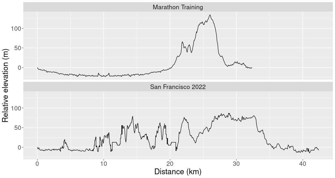
    Another limitation of total variation is that it measures total wiggliness across the whole domain rather than average wiggliness. This isn’t much of a problem when comparing runs of a similar length, but when comparing runs of different lengths, total variation can give surprising results. Below is a comparison between the Australian Alpine Ascent and the SF marathon:

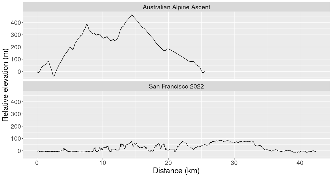
    The Australian Alpine Ascent is a 25 km run that goes up Australia’s tallest mountain. Despite the huge climbs during the Australian Alpine Ascent, the SF marathon has a higher total variation. Since the Australian Alpine Ascent was shorter, it gets a lower wiggliness score (1674 m vs 2140 m). For this comparison it would be better to divide each wiggliness score by the runs’ distance.

    Summary

    Despite these limitations, I still think that total variation is a useful metric for comparing two runs. It doesn’t tell you exactly how tough a run will be but if you already know the run’s distance and starting/finishing elevation, then the total variation helps you know what to expect.

  • A clock is a one-dimensional subgroup of the torus

    Recently, my partner and I installed a clock in our home. The clock previously belonged to my grandparents and we have owned it for a while. We hadn’t put it up earlier because the original clock movement ticked and the sound would disrupt our small studio apartment. After much procrastinating, I bought a new clock movement, replaced the old one and proudly hung up our clock.

    Our new clock. We still need to reattach the 5 and 10 which fell off when we moved.

    When I first put on the clock hands I made the mistake of not putting them both on at exactly 12 o’clock. This meant that the minute and hour hands were not synchronised. The hands were in an impossible position. At times, the minute hand was at 12 and the hour hand was between 3 and 4. It took some time for me to register my mistake as at some times of the day it can be hard to tell that the hands are out of sync (how often do you look at a clock at 12:00 exactly?). Fortunately, I did notice the mistake and we have a correct clock. Now I can’t help noticing when others make the same mistake such as in this piece of clip art.

    An incorrect clock where the minute hand points to 6 but the hour hand is exactly at 10. From 30 Clipart – Clock Face Clip Art @clipartmax.com

    After fixing the clock, I was still thinking about how only some clock hand positions correspond to actual times. This led me to think “a clock is a one-dimensional subgroup of the torus”. Let me explain why.

    The torus

    The minute and hour hands on a clock can be thought of as two points on two different circles. For instance, if the time is 9:30, then the minute hand corresponds to a point at the very bottom of the circle and the hour hand corresponds to a point 15 degrees clockwise of the leftmost point of the circle. As a clock goes through a 12 hour cycle the minute-hand-point goes around the circle 12 times and the hour-hand-point goes around the circle once. This is shown below.

    The blue point goes around its blue circle in time with the minute hand on the clock in the middle. The red point goes around its red circle in time with the hour hand.

    If you take the collection of all pairs of points on a circle you get what mathematicians call a torus. The torus is a geometric shape that looks like the surface of a donut. The torus is defined as the Cartesian product of two circles. That is, a single point on the torus corresponds to two points on two different circles. A torus is plotted below.

    The green surface above is a torus. The black lines aren’t a part of the torus, they are just there to help the visualisation.

    To understand the torus, it’s helpful to consider a more familiar example, the 2-dimensional plane. If we have points \(x\) and \(y\) on two different lines, then we can produce the point \((x,y)\) in the two dimensional plane. Likewise, if we have a point \(p\) and a point \(q\) on two different circles, then we can produce a point \((p,q)\) on the torus. Both of these concepts are illustrated below. I have added two circles to the torus which are analogous to the x and y axes of the plane. The blue and red points on the blue and red circle produce the black point on the torus.

    Mapping the clock to the torus

    The points on the torus are in one-to-one correspondence with possible arrangements of the two clock hands. However, as I learnt putting up our clock, not all arrangements of clock hands correspond to an actual time. This means that only some points on the torus correspond to an actual time but how can we identify these points?

    Keeping with our previous convention, let’s use the blue circle to represent the position of the minute hand and the red circle to represent the position of the hour hand. This means that the point where the two circles meet corresponds to 12 o’clock.

    The point where the two circles meet corresponds to both hands pointing to 12, that is, 12 o’clock.

    There are eleven other points on the red line that correspond to the other times when the minute hand is at 12. That is, there’s a point for 1 o’clock, 2 o’clock, 3 o’clock and so on. Once we add in those points, our torus looks like this:

    Each black dot corresponds to when the minute hand is at 12. That is, the dots represent 12 o’clock, 1 o’clock, 2 o’clock and so on.

    Finally, we have to join these points together. We know that when the hour hand moves from 12 to 1, the minute hand does one full rotation. This means that we have to join the black points by making one full rotation in the direction of the blue circle. The result is the black curve below that snakes around the torus.

    Points on the black curve correspond to actual times on the clock.

    The picture above should explain most of this blog’s title – “a clock is a one-dimensional subgroup of the torus”. We now know what the torus is and why certain points on the torus correspond to positions of the hands on a clock. We can see that these “clock points” correspond to a line that snakes around the torus. While the torus is a surface and hence two dimensional, the line is one-dimensional. The last missing part is the word “subgroup”. I won’t go into the details here but the torus has some extra structure that makes it something called a group. Our map from the clock to the torus interacts nicely with this structure and this makes the black line a “subgroup”.

    Another perspective

    While the above pictures of the torus are pretty, they can be a bit hard to understand and hard to draw. Mathematicians have another perspective of the torus that is often easier to work with. Imagine that you have a square sheet of rubber. If you rolled up the rubber and joined a pair of opposite sides, you would get a rubber tube. If you then bent the tube to join the opposite sides again, you would get a torus! The gif bellow illustrates this idea

    By joining opposite sides, we can turn a square into a torus. This gif is taken from https://en.wikipedia.org/wiki/Torus

    This means that we can simply view the torus as a square. We just have to remember that the opposite sides of the squares have been glued together. So like a game of snake on a phone, if you leave the top of the square, you come out at the same place on the bottom of the square. If we use this idea to redraw our torus it now looks like this:

    A drawing of a flat torus. To make a donut shaped torus, the two red lines and then the two blue lines have to be glued together. As before, the blue line corresponds to the minute hand and the red line to the hour hand. When we glue the opposite sides of this square, the four corners all get glued together. This point is where the two circles intersect and corresponds to 12 o’clock.

    As before we can draw in the other points when the minute hand is at 12. These points correspond to 1 o’clock, 2 o’clock, 3 o’clock…

    Each black dot corresponds to a time when the minute hand is at 12. Remember that each dot on the top is actually the same point as the corresponding dot on the bottom. These opposite points get glued together when we turn the square into a torus.

    Finally we can draw in all the other times on the clock. This is the result:

    Points on the black line correspond to actual times on the clock. Although it looks like there are 12 different lines, there is actually only one line once we glue the opposite sides together.

    One nice thing about this picture is that it can help us answer a classic riddle. In a 12-hour cycle, how many times are the minute and hour hands on top of each other? We can answer this riddle by adding a second line to the above square. The bottom-left to top-right diagonal is the collection of all hand positions where the two hands are on top of each other. Let’s add that line in green and add the points where this new line intersects the black line.

    The green line is the collection of all hand positions when the two hands are pointing in the same direction. The black points are where the green and black lines intersect each other.

    The points where the green and black lines intersect are hand positions where the clock hands are directly on top of each other and which correspond to actual times. Thus we can count that there are exactly 11 times when the hands are on top of each other in a 12-hour cycle. It might look like there are 12 such times but we have to remember that the corners of the square are all the same point on the torus.

    Adding the second hand

    So far I have ignored the second hand on the clock. If we included the second hand, we would have three points on three different circles. The corresponding geometric object is a 3-dimensional torus. The 3-dimensional torus is what you get when you take a cube and glue together the three pairs of opposite faces (don’t worry if you have trouble visualising such a shape!).

    The points on the 3-dimensional torus which correspond to actual times will again be a line that wraps around the 3-dimensional torus. You could use this line to find out how many times the three hands are all on top of each other! Let me know if you work it out.

    I hope that if you’re ever asked to define a clock, you’d at least consider saying “a clock is a one-dimensional subgroup of the torus” and you could even tell them which subgroup!

  • The Singular Value Decomposition (SVD)

    The singular value decomposition (SVD) is a powerful matrix decomposition. It is used all the time in statistics and numerical linear algebra. The SVD is at the heart of the principal component analysis, it demonstrates what’s going on in ridge regression and it is one way to construct the Moore-Penrose inverse of a matrix. For more SVD love, see the tweets below.

    A tweet by Women in Statistics and Data Science about the SVD.
    The full thread is here https://twitter.com/WomenInStat/status/1285610321747611653?s=20&t=Elj62mGSc9gINHvbwt82Zw

    In this post I’ll define the SVD and prove that it always exists. At the end we’ll look at some pictures to better understand what’s going on.

    Definition

    Let \(X\) be a \(n \times p\) matrix. We will define the singular value decomposition first in the case \(n \ge p\). The SVD consists of three matrix \(U \in \mathbb{R}^{n \times p}, \Sigma \in \mathbb{R}^{p \times p}\) and \(V \in \mathbb{R}^{p \times p}\) such that \(X = U\Sigma V^T\). The matrix \(\Sigma\) is required to be diagonal with non-negative diagonal entries \(\sigma_1 \ge \sigma_2 \ge \ldots \ge \sigma_p \ge 0\). These numbers are called the singular values of \(X\). The matrices \(U\) and \(V\) are required to orthogonal matrices so that \(U^TU=V^TV = I_p\), the \(p \times p\) identity matrix. Note that since \(V\) is square we also have \(VV^T=I_p\) however we won’t have \(UU^T = I_n\) unless \(n = p\).

    In the case when \(n \le p\), we can define the SVD of \(X\) in terms of the SVD of \(X^T\). Let \(\widetilde{U} \in \mathbb{R}^{p \times n}, \widetilde{\Sigma} \in \mathbb{R}^{n \times n}\) and \(\widetilde{V} \in \mathbb{R}^{n \times n}\) be the SVD of \(X^T\) so that \(X^T=\widetilde{U}\widetilde{\Sigma}\widetilde{V}^T\). The SVD of \(X\) is then given by transposing both sides of this equation giving \(U = \widetilde{V}, \Sigma = \widetilde{\Sigma}^T=\widetilde{\Sigma}\) and \(V = \widetilde{U}\).

    Construction

    The SVD of a matrix can be found by iteratively solving an optimisation problem. We will first describe an iterative procedure that produces matrices \(U \in \mathbb{R}^{n \times p}, \Sigma \in \mathbb{R}^{p \times p}\) and \(V \in \mathbb{R}^{p \times p}\). We will then verify that \(U,\Sigma \) and \(V\) satisfy the defining properties of the SVD.

    We will construct the matrices \(U\) and \(V\) one column at a time and we will construct the diagonal matrix \(\Sigma\) one entry at a time. To construct the first columns and entries, recall that the matrix \(X\) is really a linear function from \(\mathbb{R}^p\) to \(\mathbb{R}^n\) given by \(v \mapsto Xv\). We can thus define the operator norm of \(X\) via

    \(\Vert X \Vert = \sup\left\{ \|Xv\|_2 : \|v\|_2 =1\right\},\)

    where \(\|v\|_2\) represents the Euclidean norm of \(v \in \mathbb{R}^p\) and \(\|Xv\|_2\) is the Euclidean norm of \(Xv \in \mathbb{R}^n\). The set of vectors \(\{v \in \mathbb{R} : \|v\|_2 = 1 \}\) is a compact set and the function \(v \mapsto \|Xv\|_2\) is continuous. Thus, the supremum used to define \(\Vert X \Vert\) is achieved at some vector \(v_1 \in \mathbb{R}^p\). Define \(\sigma_1 = \|X v_1\|_2\). If \(\sigma_1 \neq 0\), then define \(u_1 = Xv_1/\sigma_1 \in \mathbb{R}^n\). If \(\sigma_1 = 0\), then define \(u_1\) to be an arbitrary vector in \(\mathbb{R}^n\) with \(\|u\|_2 = 1\). To summarise we have

    • \(v_1 \in \mathbb{R}^p\) with \(\|v_1\|_2 = 1\).
    • \(\sigma_1 = \|X\| = \|Xv_1\|_2\).
    • \(u_1 \in \mathbb{R}^n\) with \(\|u_1\|_2=1\) and \(Xv_1 = \sigma_1u_1\).

    We have now started to fill in our SVD. The number \(\sigma_1 \ge 0\) is the first singular value of \(X\) and the vectors \(v_1\) and \(u_1\) will be the first columns of the matrices \(V\) and \(U\) respectively.

    Now suppose that we have found the first \(k\) singular values \(\sigma_1,\ldots,\sigma_k\) and the first \(k\) columns of \(V\) and \(U\). If \(k = p\), then we are done. Otherwise we repeat a similar process.

    Let \(v_1,\ldots,v_k\) and \(u_1,\ldots,u_k\) be the first \(k\) columns of \(V\) and \(U\). The vectors \(v_1,\ldots,v_k\) split \(\mathbb{R}^p\) into two subspaces. These subspaces are \(S_1 = \text{span}\{v_1,\ldots,v_k\}\) and \(S_2 = S_1^\perp\), the orthogonal compliment of \(S_1\). By restricting \(X\) to \(S_2\) we get a new linear map \(X_{|S_2} : S_2 \to \mathbb{R}^n\). Like before, the operator norm of \(X_{|S_2}\) is defined to be

    \(\|X_{|S_2}\| = \sup\{\|X_{|S_2}v\|_2:v \in S_2, \|v\|_2=1\}\).

    Since \(S_2 = \text{span}\{v_1,\ldots,v_k\}^\perp\) we must have

    \(\|X_{|S_2}\| = \sup\{\|Xv\|_2:v \in \mathbb{R}^p, \|v\|_2=1, v_j^Tv = 0 \text{ for } j=1,\ldots,k\}.\)

    The set \(\{v \in \mathbb{R}^p : \|v\|_2=1, v_j^Tv=0\text{ for } j=1,\ldots,k\}\) is a compact set and thus there exists a vector \(v_{k+1}\) such that \(\|Xv_{k+1}\|_2 = \|X_{|S_2}\|\). As before define \(\sigma_{k+1} = \|Xv_{k+1}\|_2\) and \(u_{k+1} = Xv_{k+1}/\sigma_{k+1}\) if \(\sigma_{k+1}\neq 0\). If \(\sigma_{k+1} = 0\), then define \(u_{k+1}\) to be any vector in \(\mathbb{R}^{n}\) that is orthogonal to \(u_1,u_2,\ldots,u_k\).

    This process repeats until eventually \(k = p\) and we have produced matrices \(U \in \mathbb{R}^{n \times p}, \Sigma \in \mathbb{R}^{p \times p}\) and \(V \in \mathbb{R}^{p \times p}\). In the next section, we will argue that these three matrices satisfy the properties of the SVD.

    Correctness

    The defining properties of the SVD were given at the start of this post. We will see that most of the properties follow immediately from the construction but one of them requires a bit more analysis. Let \(U = [u_1,\ldots,u_p]\), \(\Sigma = \text{diag}(\sigma_1,\ldots,\sigma_p)\) and \(V= [v_1,\ldots,v_p]\) be the output from the above construction.

    First note that by construction \(v_1,\ldots, v_p\) are orthogonal since we always had \(v_{k+1} \in \text{span}\{v_1,\ldots,v_k\}^\perp\). It follows that the matrix \(V\) is orthogonal and so \(V^TV=VV^T=I_p\).

    The matrix \(\Sigma\) is diagonal by construction. Furthermore, we have that \(\sigma_{k+1} \le \sigma_k\) for every \(k\). This is because both \(\sigma_k\) and \(\sigma_{k+1}\) were defined as maximum value of \(\|Xv\|_2\) over different subsets of \(\mathbb{R}^p\). The subset for \(\sigma_k\) contained the subset for \(\sigma_{k+1}\) and thus \(\sigma_k \ge \sigma_{k+1}\).

    We’ll next verify that \(X = U\Sigma V^T\). Since \(V\) is orthogonal, the vectors \(v_1,\ldots,v_p\) form an orthonormal basis for \(\mathbb{R}^p\). It thus suffices to check that \(Xv_k = U\Sigma V^Tv_k\) for \(k = 1,\ldots,p\). Again by the orthogonality of \(V\) we have that \(V^Tv_k = e_k\), the \(k^{th}\) standard basis vector. Thus,

    \(U\Sigma V^Tv_k = U\Sigma e_k = U\sigma_k e_k = \sigma_k u_k.\)

    Above, we used that \(\Sigma\) was a diagonal matrix and that \(u_k\) is the \(k^{th}\) column of \(U\). If \(\sigma_k \neq 0\), then \(\sigma_k u_k = Xv_k\) by definition. If \(\sigma_k =0\), then \(\|Xv_k\|_2=0\) and so \(Xv_k = 0 = \sigma_ku_k\) also. Thus, in either case, \(U\Sigma V^Tv_k = Xv_k\) and so \(U\Sigma V^T = X\).

    The last property we need to verify is that \(U\) is orthogonal. Note that this isn’t obvious. At each stage of the process, we made sure that \(v_{k+1} \in \text{span}\{v_1,\ldots,v_k\}^\perp\). However, in the case that \(\sigma_{k+1} \neq 0\), we simply defined \(u_{k+1} = Xv_{k+1}/\sigma_{k+1}\). It is not clear why this would imply that \(u_{k+1}\) is orthogonal to \(u_1,\ldots,u_k\).

    It turns out that a geometric argument is needed to show this. The idea is that if \(u_{k+1}\) was not orthogonal to \(u_j\) for some \(j \le k\), then \(v_j\) couldn’t have been the value that maximises \(\|Xv\|_2\).

    Let \(u_{k}\) and \(u_j\) be two columns of \(U\) with \(j < k\) and \(\sigma_j,\sigma_k > 0\). We wish to show that \(u_j^Tu_k = 0\). To show this we will use the fact that \(v_j\) and \(v_k\) are orthonormal and perform “polar-interpolation“. That is, for \(\lambda \in [0,1]\), define

    \(v_\lambda = \sqrt{1-\lambda}\cdot v_{j}-\sqrt{\lambda} \cdot v_k.\)

    Since \(v_{j}\) and \(v_k\) are orthogonal, we have that

    \(\|v_\lambda\|_2^2 = (1-\lambda)\|v_{j}\|_2^2+\lambda\|v_k\|_2^2 = (1-\lambda)+\lambda = 1.\)

    Furthermore \(v_\lambda\) is orthogonal to \(v_1,\ldots,v_{j-1}\). Thus, by definition of \(v_j\),

    \(\|Xv_\lambda\|_2^2 \le \sigma_j^2 = \|Xv_j\|_2^2.\)

    By the linearity of \(X\) and the definitions of \(u_j,u_k\),

    \(\|Xv_\lambda\|_2^2 = \|\sqrt{1-\lambda}\cdot Xv_j+\sqrt{\lambda}\cdot Xv_{k+1}\|_2^2 = \|\sigma_j\sqrt{1-\lambda}\cdot u_j+\sigma_{k+1}\sqrt{\lambda}\cdot u_{k+1}\|_2^2\).

    Since \(Xv_j = \sigma_ju_j\) and \(Xv_{k+1}=\sigma_{k+1}u_{k+1}\), we have

    \((1-\lambda)\sigma_j^2 + 2\sqrt{\lambda(1-\lambda)}\cdot \sigma_1\sigma_2 u_j^Tu_{k}+\lambda\sigma_k^2 = \|Xv_\lambda\|_2^2 \le \sigma_j^2\)

    Rearranging and dividing by \(\sqrt{\lambda}\) gives,

    \(2\sqrt{1-\lambda}\cdot \sigma_1\sigma_2 u_j^Tu_k \le \sqrt{\lambda}\cdot(\sigma_j^2-\sigma_k^2).\) for all \(\lambda \in (0,1]\)

    Taking \(\lambda \searrow 0\) gives \(u_j^Tu_k \le 0\). Performing the same polar interpolation with \(v_\lambda’ = \sqrt{1-\lambda}v_j – \sqrt{\lambda}v_k\) shows that \(-u_j^Tu_k \le 0\) and hence \(u_j^Tu_k = 0\).

    We have thus proved that \(U\) is orthogonal. This proof is pretty “slick” but it isn’t very illuminating. To better demonstrate the concept, I made an interactive Desmos graph that you can access here.

    This graph shows example vectors \(u_j, u_k \in \mathbb{R}^2\). The vector \(u_j\) is fixed at \((1,0)\) and a quarter circle of radius \(1\) is drawn. Any vectors \(u\) that are outside this circle have \(\|u\|_2 > 1 = \|u_j\|_2\).

    The vector \(u_k\) can be moved around inside this quarter circle. This can be done either cby licking and dragging on the point or changing that values of \(a\) and \(b\) on the left. The red curve is the path of

    \(\lambda \mapsto \sqrt{1-\lambda}\cdot u_j+\sqrt{\lambda}\cdot u_k\).

    As \(\lambda\) goes from \(0\) to \(1\), the path travels from \(u_j\) to \(u_k\).

    Note that there is a portion of the red curve near \(u_j\) that is outside the black circle. This corresponds to a small value of \(\lambda > 0\) that results in \(\|X v_\lambda\|_2 > \|Xv_j\|_2\) contradicting the definition of \(v_j\). By moving the point \(u_k\) around in the plot you can see that this always happens unless \(u_k\) lies exactly on the y-axis. That is, unless \(u_k\) is orthogonal to \(u_j\).

  • Double cosets and contingency tables

    Like my previous post, this blog is also motivated by a comment by Professor Persi Diaconis in his recent Stanford probability seminar. The seminar was about a way of “collapsing” a random walk on a group to a random walk on the set of double cosets. In this post, I’ll first define double cosets and then go over the example Professor Diaconis used to make us probabilists and statisticians more comfortable with all the group theory he was discussing.

    Double cosets

    Let \(G\) be a group and let \(H\) and \(K\) be two subgroups of \(G\). For each \(g \in G\), the \((H,K)\)-double coset containing \(g\) is defined to be the set

    \(HgK = \{hgk : h \in H, k \in K\}\)

    To simplify notation, we will simply write double coset instead of \((H,K)\)-double coset. The double coset of \(g\) can also be defined as the equivalence class of \(g\) under the relation

    \(g \sim g’ \Longleftrightarrow g’ = hgk\) for some \(h \in H\) and \(g \in G\)

    Like regular cosets, the above relation is indeed an equivalence relation. Thus, the group \(G\) can be written as a disjoint union of double cosets. The set of all double cosets of \(G\) is denoted by \(H\backslash G / K\). That is,

    \(H\backslash G /K = \{HgK : g \in G\}\)

    Note that if we take \(H = \{e\}\), the trivial subgroup, then the double cosets are simply the left cosets of \(K\), \(G / K\). Likewise if \(K = \{e\}\), then the double cosets are the right cosets of \(H\), \(H \backslash G\). Thus, double cosets generalise both left and right cosets.

    Double cosets in \(S_n\)

    Fix a natural number \(n > 0\). A partition of \(n\) is a finite sequence \(a = (a_1,a_2,\ldots, a_I)\) such that \(a_1,a_2,\ldots, a_I \in \mathbb{N}\), \(a_1 \ge a_2 \ge \ldots a_I > 0\) and \(\sum_{i=1}^I a_i = n\). For each partition of \(n\), \(a\), we can form a subgroup \(S_a\) of the symmetric group \(S_n\). The subgroup \(S_a\) contains all permutations \(\sigma \in S_n\) such that \(\sigma\) fixes the sets \(A_1 = \{1,\ldots, a_1\}, A_2 = \{a_1+1,\ldots, a_1 + a_2\},\ldots, A_I = \{n – a_I +1,\ldots, n\}\). Meaning that \(\sigma(A_i) = A_i\) for all \(1 \le i \le I\). Thus, a permutation \(\sigma \in S_a\) must individually permute the elements of \(A_1\), the elements of \(A_2\) and so on. This means that, in a natural way,

    \(S_a \cong S_{a_1} \times S_{a_2} \times \ldots \times S_{a_I}\)

    If we have two partitions \(a = (a_1,a_2,\ldots, a_I)\) and \(b = (b_1,b_2,\ldots,b_J)\), then we can form two subgroups \(H = S_a\) and \(K = S_b\) and consider the double cosets \(H \backslash G / K = S_a \backslash S_n / S_b\). The claim made in the seminar was that the double cosets are in one-to-one correspondence with \(I \times J\) contingency tables with row sums equal to \(a\) and column sums equal to \(b\). Before we explain this correspondence and properly define contingency tables, let’s first consider the cases when either \(H\) or \(K\) is the trivial subgroup.

    Left cosets in \(S_n\)

    Note that if \(a = (1,1,\ldots,1)\), then \(S_a\) is the trivial subgroup and, as noted above, \(S_a \backslash S_n / S_b\) is simply equal to \(S_n / S_b\). We will see that the cosets in \(S_n/S_b\) can be described by forgetting something about the permutations in \(S_n\).

    We can think of the permutations in \(S_n\) as all the ways of drawing without replacement \(n\) balls labelled \(1,2,\ldots, n\). We can think of the partition \(b = (b_1,b_2,\ldots,b_J)\) as a colouring of the \(n\) balls by \(J\) colours. We colour balls \(1,2,\ldots, b_1\) by the first colour \(c_1\), then we colour \(b_1+1,b_1+2,\ldots, b_1+b_2\) the second colour \(c_2\) and so on until we colour \(n-b_J+1, n-b_J+2,\ldots, n\) the final colour \(c_J\). Below is an example when \(n\) is equal to 6 and \(b = (3,2,1)\).

    The first three balls are coloured green, the next two are coloured red and the last ball is coloured blue.

    Note that a permutation \(\sigma \in S_n\) is in \(S_b\) if and only if we draw the balls by colour groups, i.e. we first draw all the balls with colour \(c_1\), then we draw all the balls with colour \(c_2\) and so on. Thus, continuing with the previous example, the permutation \(\sigma_1\) below is in \(S_b\) but \(\sigma_2\) is not in \(S_b\).

    The permutation \(\sigma_1\) is in \(S_b\) because the colours are in their original order but \(\sigma_1\) is not in \(S_b\) because the colours are rearranged.

    It turns out that we can think of the cosets in \(S_n \setminus S_b\) as what happens when we “forget” the labels \(1,2,\ldots,n\) and only remember the colours of the balls. By “forgetting” the labels we mean only paying attention to the list of colours. That is for all \(\sigma_1,\sigma_2 \in S_n\), \(\sigma_1 S_b = \sigma_2 S_b\) if and only if the list of colours from the draw \(\sigma_1\) is the same as the list of colours from the draw \(\sigma_2\). Thus, the below two permutations define the same coset of \(S_b\)

    When we forget the labels and only remember the colours, the permutations \(\sigma_1\) and \(\sigma_2\) look the same and thus are in the same left coset of \(S_b\).

    To see why this is true, note that \(\sigma_1 S_b = \sigma_2 S_b\) if and only if \(\sigma_2 = \sigma_1 \circ \tau\) for some \(\tau \in S_b\). Furthermore, \(\tau \in S_b\) if and only if \(\tau\) maps each colour group to itself. Recall that function composition is read right to left. Thus, the equation \(\sigma_2 = \sigma_1 \circ \tau\) means that if we first relabel the balls according to \(\tau\) and then draw the balls according to \(\sigma_1\), then we get the result as just drawing by \(\sigma_2\). That is, \(\sigma_2 = \sigma_1 \circ \tau\) for some \(\tau \in S_b\) if and only if drawing by \(\sigma_2\) is the same as first relabelling the balls within each colour group and then drawing the balls according to \(\sigma_1\). Thus, \(\sigma_1 S_b = \sigma_2 S_b\), if and only if when we forget the labels of the balls and only look at the colours, \(\sigma_1\) and \(\sigma_2\) give the same list of colours. This is illustrated with our running example below.

    If we permute the balls according to \(\tau \in S_b\) and the draw according to \(\sigma_1\), then the resulting draw is the same as if we had not permuted and drawn according to \(\sigma_2\). That is, \(\sigma_2 = \sigma_1 \circ \tau\).

    Right cosets of \(S_n\)

    Typically, the subgroup \(S_a\) is not a normal subgroup of \(S_n\). This means that the right coset \(S_a \sigma\) will not equal the left coset \(\sigma S_a\). Thus, colouring the balls and forgetting the labelling won’t describe the right cosets \(S_a \backslash S_n\). We’ll see that a different type of forgetting can be used to describe \(S_a \backslash S_n = \{S_a\sigma : \sigma \in S_n\}\).

    Fix a partition \(a = (a_1,a_2,\ldots,a_I)\) and now, instead of considering \(I\) colours, think of \(I\) different people \(p_1,p_2,\ldots,p_I\). As before, a permutation \(\sigma \in S_n\) can be thought of drawing \(n\) balls labelled \(1,\ldots,n\) without replacement. We can imagine giving the first \(a_1\) balls drawn to person \(p_1\), then giving the next \(a_2\) balls to the person \(p_2\) and so on until we give the last \(a_I\) balls to person \(p_I\). An example with \(n = 6\) and \(a = (2,2,2)\) is drawn below.

    Person \(p_1\) receives the ball labelled by 6 followed by the ball labelled 3, person \(p_2\) receives ball 2 and then ball 1 and finally person \(p_3\) receives ball 4 followed by ball 5.

    Note that \(\sigma \in S_a\) if and only if person \(p_i\) receives the balls with labels \(\sum_{k=0}^{i-1}a_k+1,\sum_{k=0}^{i-1}a_k+2,\ldots, \sum_{k=0}^i a_k\) in any order. Thus, in the below example \(\sigma_1 \in S_a\) but \(\sigma_2 \notin S_a\).

    When the balls are drawn according to \(\sigma_1\), person \(p_i\) receives the balls with labels \(2i-1\) and \(2i\), and thus \(\sigma_1 \in S_a\). On the other hand, if the balls are drawn according to \(\sigma_2\), the people receive different balls and thus \(\sigma_2 \notin S_a\).

    It turns out the cosets \(S_a \backslash S_n\) are exactly determined by “forgetting” the order in which each person \(p_i\) received their balls and only remembering which balls they received. Thus, the two permutation below belong to the same coset in \(S_a \backslash S_n\).

    When we forget the order in which each person receive their balls, the permutations \(\sigma_1\) and \(\sigma_2\) become the same and thus \(S_a \sigma_1 = S_a \sigma_2\). Note that if we coloured the balls according to the permutation \(a = (a_1,\ldots,a_I)\), then we could see that \(\sigma_1 S_a \neq \sigma_2 S_a\).

    To see why this is true in general, consider two permutations \(\sigma_1,\sigma_2\). The permutations \(\sigma_1,\sigma_2\) result in each person \(p_i\) receiving the same balls if and only if after \(\sigma_1\) we can apply a permutation \(\tau\) that fixes each subset \(A_i = \left\{\sum_{k=0}^{i-1}a_k+1,\ldots, \sum_{k=0}^i a_k\right\}\) and get \(\sigma_2\). That is, \(\sigma_1\) and \(\sigma_2\) result in each person \(p_i\) receiving the same balls if and only if \(\sigma_2 = \tau \circ \sigma_1\) for some \(\tau \in S_a\). Thus, \(\sigma_1,\sigma_2\) are the same after forgetting the order in which each person received their balls if and only if \(S_a \sigma_1 = S_a \sigma_2\). This is illustrated below,

    If we first draw the balls according to \(\sigma_1\) and then permute the balls according to \(\tau\), then the resulting draw is the same as if we had drawn according to \(\sigma_2\) and not permuted afterwards. That is, \(\sigma_2 = \tau \circ \sigma_1 \).

    We can thus see why \(S_a \backslash S_n \neq S_n / S_a\). A left coset \(\sigma S_a\) correspond to pre-composing \(\sigma\) with elements of \(S_a\) and a right cosets \(S_a\sigma\) correspond to post-composing \(\sigma\) with elements of \(S_a\).

    Contingency tables

    With the last two sections under our belts, describing the double cosets \(S_a \backslash S_n / S_b\) is straight forward. We simply have to combine our two types of forgetting. That is, we first colour the \(n\) balls with \(J\) colours according to \(b = (b_1,b_2,\ldots,b_J)\). We then draw the balls without replace and give the balls to \(I\) different people according \(a = (a_1,a_2,\ldots,a_I)\). We then forget both the original labels and the order in which each person received their balls. That is, we only remember the number of balls of each colour each person receives. Describing the double cosets by “double forgetting” is illustrated below with \(a = (2,2,2)\) and \(b = (3,2,1)\).

    The permutations \(\sigma_1\) and \(\sigma_2\) both result in person \(p_1\) receiving one green ball and one blue ball. The two permutations also results in \(p_2\) and \(p_3\) both receiving one green ball and one red ball. Thus, \(\sigma_1\) and \(\sigma_2\) are both in the same \((S_a,S_b)\)-double coset. Note however that \(\sigma_1 S_b \neq \sigma_2 S_b\) and \(S_a\sigma_1 \neq S_a \sigma_2\).

    The proof that double forgetting does indeed describe the double cosets is simply a combination of the two arguments given above. After double forgetting, the number of balls given to each person can be recorded in an \(I \times J\) table. The \(N_{ij}\) entry of the table is simply the number of balls person \(p_i\) receives of colour \(c_j\). Two permutations are the same after double forgetting if and only if they produce the same table. For example, \(\sigma_1\) and \(\sigma_2\) above both produce the following table

    Green (\(c_1\)) Red (\(c_2\))Blue (\(c_3\))Total
    Person \(p_1\)1012
    Person \(p_2\)1102
    Person \(p_3\)1102
    Total3216

    By the definition of how the balls are coloured and distributed to each person we must have for all \(1 \le i \le I\) and \(1 \le j \le J\)

    \(\sum_{j=1}^J N_{ij} = a_i \) and \(\sum_{i=1}^I N_{ij} = b_j\)

    An \(I \times J\) table with entries \(N_{ij} \in \{0,1,2,\ldots\}\) satisfying the above conditions is called a contingency table. Given such a contingency table with entries \(N_{ij}\) where the rows sum to \(a\) and the columns sum to \(b\), there always exists at least one permutation \(\sigma\) such that \(N_{ij}\) is the number of balls received by person \(p_i\) of colour \(c_i\). We have already seen that two permutations produce the same table if and only if they are in the same double coset. Thus, the double cosets \(S_a \backslash S_n /S_b\) are in one-to-one correspondence with such contingency tables.

    The hypergeometric distribution

    I would like to end this blog post with a little bit of probability and relate the contingency tables above to the hyper geometric distribution. If \(a = (m, n-m)\) for some \(m \in \{0,1,\ldots,n\}\), then the contingency tables described above have two rows and are determined by the values \(N_{11}, N_{12},\ldots, N_{1J}\) in the first row. The numbers \(N_{1j}\) are the number of balls of colour \(c_j\) the first person receives. Since the balls are drawn without replacement, this means that if we put the uniform distribution on \(S_n\), then the vector \(Y=(N_{11}, N_{12},\ldots, N_{1J})\) follows the multivariate hypergeometric distribution. Thus, if we have a random walk on \(S_n\) that quickly converges to the uniform distribution on \(S_n\), then we could use the double cosets to get a random walk that converges to the multivariate hypergeometric distribution (although there are smarter ways to do such sampling).

  • The field with one element in a probability seminar

    Something very exciting this afternoon. Professor Persi Diaconis was presenting at the Stanford probability seminar and the field with one element made an appearance. The talk was about joint work with Mackenzie Simper and Arun Ram. They had developed a way of “collapsing” a random walk on a group to a random walk on the set of double cosets. As an illustrative example, Persi discussed a random walk on \(GL_n(\mathbb{F}_q)\) given by multiplication by a random transvection (a map of the form \(v \mapsto v + ab^Tv\), where \(a^Tb = 0\)).

    The Bruhat decomposition can be used to match double cosets of \(GL_n(\mathbb{F}_q)\) with elements of the symmetric group \(S_n\). So by collapsing the random walk on \(GL_n(\mathbb{F}_q)\) we get a random walk on \(S_n\) for all prime powers \(q\). As Professor Diaconis said, you can’t stop him from taking \(q \to 1\) and asking what the resulting random walk on \(S_n\) is. The answer? Multiplication by a random transposition. As pointed sets are vector spaces over the field with one element and the symmetric groups are the matrix groups, this all fits with what’s expected of the field with one element.

    This was just one small part of a very enjoyable seminar. There was plenty of group theory, probability, some general theory and engaging examples.

    Update: I have written another post about some of the group theory from the seminar! You can read it here: Double cosets and contingency tables.