Tag: mathematics

Braids and the Yang-Baxter equation
I recently gave a talk on the Yang-Baxter equation. The focus of the talk was to state the connection between the Yang-Baxter equation and the braid relation. This connection comes from a system of interacting particles. In this post, I’ll go over part of my talk. You can access the full set of notes here.

Interacting particles

Imagine two particles on a line, each with a state that can be any element of a set \(\mathcal{X}\). Suppose that the only way particles can change their states is by interacting with each other. An interaction occurs when two particles pass by each other. We could define a function \(F : \mathcal{X} \times \mathcal{X} \to \mathcal{X} \times \mathcal{X}\) that describes how the states change after interaction. Specifically, if the first particle is in state \(x\) and the second particle is in state \(y\), then their states after interacting will be

\(F(x,y) = (F_a(x,y), F_b(x,y)) = (\text{new state of particle 1}, \text{new state of particle 2}), \)

where \(F_a,F_b : \mathcal{X} \times \mathcal{X} \to \mathcal{X}\) are the components of \(F\). Recall that the particles move past each other when they interact. Thus, to keep track of the whole system we need an element of \(\mathcal{X} \times \mathcal{X}\) to keep track of the states and a permutation \(\sigma \in S_2\) to keep track of the positions.

Three particles

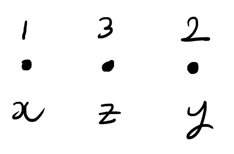
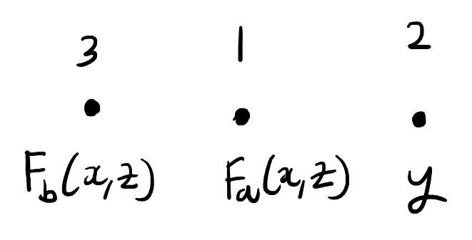
Now suppose that we have \(3\) particles labelled \(1,2,3\). As before, each particle has a state in \(\mathcal{X}\). We can thus keep track of the state of each particle with an element of \(\mathcal{X}^3\). The particles also have a position which is described by a permutation \(\sigma \in S_3\). The order the entries of \((x,y,z) \in \mathcal{X}^3\) corresponds to the labels of the particles not their positions. A possible configuration is shown below:

A possible configuration of the three particles. The above configuration is escribed as having states \((x,y,z) \in \mathcal{X}^3\) and positions \(132 \in S_3\).

As before, the particles can interact with each other. However, we’ll now add the restriction that the particles can only interact two at a time and interacting particles must have adjacent positions. When two particles interact, they swap positions and their states change according to \(F\). The state and position of the remaining particle is unchanged. For example, in the above picture we could interact particles \(1\) and \(3\). This will produce the below configuration:

The new configuration after interacting particles \(1\) and \(3\) in the first diagram. The configuration is now described by the states \(F_{13}(x,y,z) \in \mathcal{X}^3\) and the permutation \(312 \in S_3\).

To keep track of how the states of the particles change over time we will introduce three functions from \(\mathcal{X}^3\) to \(\mathcal{X}^3\). These functions are \(F_{12},F_{13},F_{23}\). The function \(F_{ij}\) is given by applying \(F\) to the \(i,j\) coordinates of \((x,y,z)\) and acting by the identity on the remaining coordinate. In symbols,

\(F_{12}(x,y,z) = (F_a(x,y), F_b(x,y), z),\)
\(F_{13}(x,y,z) = (F_a(x,z), y, F_b(x,z)),\)
\(F_{23}(x,y,z) = (x, F_a(y,z), F_b(y,z)).\)

The function \(F_{ij}\) exactly describes how the states of the three particles change when particles \(i\) and \(j\) interact. Now suppose that three particles begin in position \(123\) and states \((x,y,z)\). We cannot directly interact particles \(1\) and \(3\) since they are not adjacent. We have to pass first pass one of the particles through particle \(2\). This means that there are two ways we can interact particles \(1\) and \(3\). These are illustrated below.

The two ways of passing through particle 2 to interact particles 2 and 3.

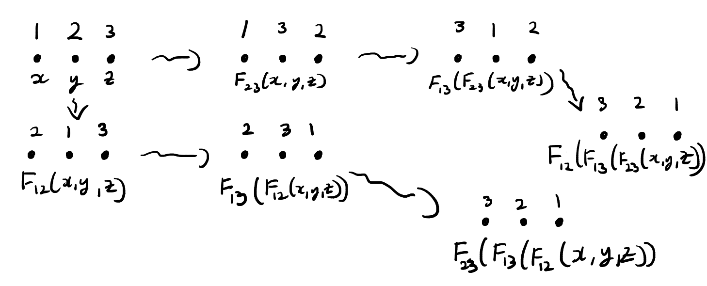
In the top chain of interactions, we first interact particles \(2\) and \(3\). In this chain of interactions, the states evolve as follows:

\((x,y,z) \to F_{23}(x,y,z) \to F_{13}(F_{23}(x,y,z)) \to F_{12}(F_{13}(F_{23}(x,y,z))).\)

In the bottom chain of interactions, we first interact particles \(1\) and \(2\). On this chain, the states evolve in a different way:

\((x,y,z) \to F_{12}(x,y,z) \to F_{13}(F_{12}(x,y,z)) \to F_{23}(F_{13}(F_{12}(x,y,z))).\)

Note that after both of these chains of interactions the particles are in position \(321\). The function \(F\) is said to solve the Yang–Baxter equation if two chains of interactions also result in the same states.

Definition: A function \(F : \mathcal{X} \times \mathcal{X} \to \mathcal{X} \times \mathcal{X}\) is a solution to the set theoretic Yang–Baxter equation if,

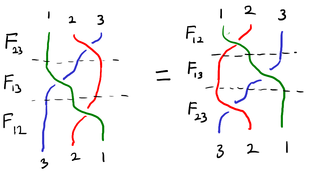
\(F_{12}\circ F_{13} \circ F_{23} = F_{23} \circ F_{13} \circ F_{12}. \)

This equation can be visualized as the “braid relation” shown below. Here the strings represent the three particles and interacting two particles corresponds to crossing one string over the other.

The braid relation.

Here are some examples of solutions to the set theoretic Yang-Baxter equation,
- The identity on \(\mathcal{X} \times \mathcal{X}\).
- The swap map, \((x,y) \mapsto (y,x)\).
- If \(f,g : \mathcal{X} \to \mathcal{X}\) commute, then the function \((x,y) \to (f(x), g(y))\) is a solution the Yang-Baxter equation.
In the full set of notes I talk about a number of extensions and variations of the Yang-Baxter equation. These include having more than three particles, allowing for the particle states to be entangle and the parametric Yang-Baxter equation.
March 12, 2023
Log-sum-exp trick with negative numbers
Suppose you want to calculate an expression of the form

\(\displaystyle{\log\left(\sum_{i=1}^n \exp(a_i) – \sum_{j=1}^m \exp(b_j)\right)},\)

where \(\sum_{i=1}^n \exp(a_i) > \sum_{j=1}^m \exp(b_j)\). Such expressions can be difficult to evaluate directly since the exponentials can easily cause overflow errors. In this post, I’ll talk about a clever way to avoid such errors.

If there were no terms in the second sum we could use the log-sum-exp trick. That is, to calculate

\(\displaystyle{\log\left(\sum_{i=1}^n \exp(a_i) \right)},\)

we set \(a=\max\{a_i : 1 \le i \le n\}\) and use the identity

\(\displaystyle{a + \log\left(\sum_{i=1}^n \exp(a_i-a)\right) = \log\left(\sum_{i=1}^n \exp(a_i)\right)}. \)

Since \(a_i \le a\) for all \(i =1,\ldots,n\), the left hand side of the above equation can be computed without the risk of overflow. To calculate,

\(\displaystyle{\log\left(\sum_{i=1}^n \exp(a_i) – \sum_{j=1}^m \exp(b_j)\right)},\)

we can use the above method to separately calculate

\(\displaystyle{A = \log\left(\sum_{i=1}^n \exp(a_i) \right)}\) and \(\displaystyle{B = \log\left(\sum_{j=1}^m \exp(b_j)\right)}.\)

The final result we want is

\(\displaystyle{\log\left(\sum_{i=1}^n \exp(a_i) – \sum_{j=1}^m \exp(b_j) \right) = \log(\exp(A) – \exp(B)) = A + \log(1-\exp(B-A))}.\)

Since $A > B$, the right hand side of the above expression can be evaluated safely and we will have our final answer.

R code

The R code below defines a function that performs the above procedure
```
# Safely compute log(sum(exp(pos)) - sum(exp(neg)))
# The default value for neg is an empty vector.

logSumExp <- function(pos, neg = c()){
  max_pos <- max(pos)
  A <- max_pos + log(sum(exp(pos - max_pos)))
  
  # If neg is empty, the calculation is done
  if (length(neg) == 0){
    return(A)
  }
  
  # If neg is non-empty, calculate B.
  max_neg <- max(neg)
  B <- max_neg + log(sum(exp(neg - max_neg)))
  
  # Check that A is bigger than B
  if (A <= B) {
    stop("sum(exp(pos)) must be larger than sum(exp(neg))")
  }
  
  # log1p() is a built in function that accurately calculates log(1+x) for |x| << 1
  return(A + log1p(-exp(B - A)))
}
```
An example

The above procedure can be used to evaulate

\(\displaystyle{\log\left(\sum_{i=1}^{200} i! – \sum_{i=1}^{500} \binom{500}{i}^2\right)}.\)

Evaluating this directly would quickly lead to errors since R (and most other programming languages) cannot compute \(200!\). However, R has the functions lfactorial() and lchoose() which can compute \(\log(i!)\) and \(\log\binom{n}{i}\) for large values of \(i\) and \(n\). We can thus put this expression in the general form at the start of this post

\(\displaystyle{\log\left(\sum_{i=1}^{200} \exp(\log(i!)) – \sum_{i=1}^{500} \exp\left(2\log\binom{500}{i}\right)\right)}.\)

The following R code thus us exactly what we want:
```
pos <- sapply(1:200, lfactorial)
neg <- sapply(1:500, function(i){2*lchoose(500, i)})

logSumExp(pos, neg)
# 863.237
```
January 21, 2023
Two sample tests as correlation tests

Suppose we have two samples \(Y_1^{(0)}, Y_2^{(0)},\ldots, Y_{n_0}^{(0)}\) and \(Y_1^{(1)},Y_2^{(1)},\ldots, Y_{n_1}^{(1)}\) and we want to test if they are from the same distribution. Many popular tests can be reinterpreted as correlation tests by pooling the two samples and introducing a dummy variable that encodes which sample each data point comes from. In this post we will see how this plays out in a simple t-test.

The equal variance t-test

In the equal variance t-test, we assume that \(Y_i^{(0)} \stackrel{\text{iid}}{\sim} \mathcal{N}(\mu_0,\sigma^2)\) and \(Y_i^{(1)} \stackrel{\text{iid}}{\sim} \mathcal{N}(\mu_1,\sigma^2)\), where \(\sigma^2\) is unknown. Our hypothesis that \(Y_1^{(0)}, Y_2^{(0)},\ldots, Y_{n_0}^{(0)}\) and \(Y_1^{(1)},Y_2^{(1)},\ldots, Y_{n_1}^{(1)}\) are from the same distribution becomes the hypothesis \(\mu_0 = \mu_1\). The test statistic is

\(t = \frac{\displaystyle \overline{Y}^{(1)} – \overline{Y}^{(0)}}{\displaystyle \hat{\sigma}\sqrt{\frac{1}{n_0}+\frac{1}{n_1}}}\),

where \(\overline{Y}^{(0)}\) and \(\overline{Y}^{(1)}\) are the two sample means. The variable \(\hat{\sigma}\) is the pooled estimate of the standard deviation and is given by

\(\hat{\sigma}^2 = \displaystyle\frac{1}{n_0+n_1-2}\left(\sum_{i=1}^{n_0}\left(Y_i^{(0)}-\overline{Y}^{(0)}\right)^2 + \sum_{i=1}^{n_1}\left(Y_i^{(1)}-\overline{Y}^{(1)}\right)^2\right)\).

Under the null hypothesis, \(t\) follows the T-distribution with \(n_0+n_1-2\) degrees of freedom. We thus reject the null \(\mu_0=\mu_1\) when \(|t|\) exceeds the \(1-\alpha/2\) quantile of the T-distribution.

Pooling the data

We can turn this two sample test into a correlation test by pooling the data and using a linear model. Let \(Y_1,\ldots,Y_{n_0}, Y_{n_0+1},\ldots,Y_{n_0+n_1}\) be the pooled data and for \(i = 1,\ldots, n_0+n_1\), define \(x_i \in \{0,1\}\) by

\(x_i = \begin{cases} 0 & \text{if } 1 \le i \le n_0,\\ 1 & \text{if } n_0+1 \le i \le n_0+n_1.\end{cases}\)

The assumptions that \(Y_i^{(0)} \stackrel{\text{iid}}{\sim} \mathcal{N}(\mu_0,\sigma^2)\) and \(Y_i^{(1)} \stackrel{\text{iid}}{\sim} \mathcal{N}(\mu_1,\sigma^2)\) can be rewritten as

\(Y_i = \beta_0+\beta_1x_i + \varepsilon_i,\)

where \(\varepsilon_i \stackrel{\text{iid}}{\sim} \mathcal{N}(0,\sigma^2)\). That is, we have expressed our modelling assumptions as a linear model. When working with this linear model, the hypothesis \(\mu_0 = \mu_1\) is equivalent to \(\beta_1 = 0\). To test \(\beta_1 = 0\) we can use the standard t-test for a coefficient in linear model. The test statistic in this case is

\(t’ = \displaystyle\frac{\hat{\beta}_1}{\hat{\sigma}_{OLS}\sqrt{(X^TX)^{-1}_{11}}},\)

where \(\hat{\beta}_1\) is the ordinary least squares estimate of \(\beta_1\), \(X \in \mathbb{R}^{(n_0+n_1)\times 2}\) is the design matrix and \(\hat{\sigma}_{OLS}\) is an estimate of \(\sigma\) given by

\(\hat{\sigma}_{OLS}^2 = \displaystyle\frac{1}{n_0+n_1-2}\sum_{i=1}^{n_0+n_1} (Y_i-\hat{Y}_i)^2,\)

where \(\hat{Y} = \hat{\beta}_0+\hat{\beta}_1x_i\) is the fitted value of \(Y_i\).

It turns out that \(t’\) is exactly equal to \(t\). We can see this by writing out the design matrix and calculating everything above. The design matrix has rows \([1,x_i]\) and is thus equal to

\(X = \begin{bmatrix} 1&x_1\\ 1&x_2\\ \vdots&\vdots\\ 1&x_{n_0}\\ 1&x_{n_0+1}\\ \vdots&\vdots\\ 1&x_{n_0+n_1}\end{bmatrix} = \begin{bmatrix} 1&0\\ 1&0\\ \vdots&\vdots\\ 1&0\\ 1&1\\ \vdots&\vdots\\ 1&1\end{bmatrix}.\)

This implies that

\(X^TX = \begin{bmatrix} n_0+n_1 &n_1\\n_1&n_1 \end{bmatrix},\)

And therefore,

\((X^TX)^{-1} = \frac{1}{(n_0+n_1)n_1-n_1^2}\begin{bmatrix} n_1 &-n_1\\-n_1&n_0+n_1 \end{bmatrix} = \frac{1}{n_0n_1}\begin{bmatrix} n_1&-n_1\\-n_1&n_0+n_1\end{bmatrix} =\begin{bmatrix} \frac{1}{n_0}&-\frac{1}{n_0}\\-\frac{1}{n_0}&\frac{1}{n_0}+\frac{1}{n_1}\end{bmatrix} .\)

Thus, \((X^TX)^{-1}_{11} = \frac{1}{n_0}+\frac{1}{n_1}\). So,

\(t’ = \displaystyle\frac{\hat{\beta}_1}{\hat{\sigma}_{OLS}\sqrt{\frac{1}{n_0}+\frac{1}{n_1}}},\)

which is starting to like \(t\) from the two-sample test. Now

\(X^TY = \begin{bmatrix} \displaystyle\sum_{i=1}^{n_0+n_1} Y_i\\ \displaystyle \sum_{i=n_0+1}^{n_0+n_1} Y_i \end{bmatrix} = \begin{bmatrix} n_0\overline{Y}^{(0)} + n_1\overline{Y}^{(1)}\\ n_1\overline{Y}^{(1)} \end{bmatrix}.\)

And so

\(\hat{\beta} = (X^TX)^{-1}X^TY = \begin{bmatrix} \frac{1}{n_0}&-\frac{1}{n_0}\\-\frac{1}{n_0}&\frac{1}{n_0}+\frac{1}{n_1}\end{bmatrix}\begin{bmatrix} n_0\overline{Y}^{(0)} + n_1\overline{Y}^{(1)}\\ n_1\overline{Y}^{(1)} \end{bmatrix}=\begin{bmatrix} \overline{Y}^{(0)}\\ \overline{Y}^{(1)} -\overline{Y}^{(0)}\end{bmatrix}.\)

Thus, \(\hat{\beta}_1 = \overline{Y}^{(1)} -\overline{Y}^{(0)}\) and

\(t’ = \displaystyle\frac{\overline{Y}^{(1)}-\overline{Y}^{(0)}}{\hat{\sigma}_{OLS}\sqrt{\frac{1}{n_0}+\frac{1}{n_1}}}.\)

This means to show that \(t’ = t\), we only need to show that \(\hat{\sigma}_{OLS}^2=\hat{\sigma}^2\). To do this, note that the fitted values \(\hat{Y}\) are equal to

\(\displaystyle\hat{Y}_i=\hat{\beta}_0+x_i\hat{\beta}_1 = \begin{cases} \overline{Y}^{(0)} & \text{if } 1 \le i \le n_0,\\ \overline{Y}^{(1)} & \text{if } n_0+1\le i \le n_0+n_1\end{cases}.\)

Thus,

\(\hat{\sigma}^2_{OLS} = \displaystyle\frac{1}{n_0+n_1-2}\sum_{i=1}^{n_0+n_1}\left(Y_i-\hat{Y}_i\right)^2=\displaystyle\frac{1}{n_0+n_1-2}\left(\sum_{i=1}^{n_0}\left(Y_i^{(0)}-\overline{Y}^{(0)}\right)^2 + \sum_{i=1}^{n_1}\left(Y_i^{(1)}-\overline{Y}^{(1)}\right)^2\right),\)

Which is exactly \(\hat{\sigma}^2\). Therefore, \(t’=t\) and the two sample t-test is equivalent to a correlation test.

The Friedman-Rafsky test

In the above example, we saw that the two sample t-test was a special case of the t-test for regressions. This is neat but both tests make very strong assumptions about the data. However, the same thing happens in a more interesting non-parametric setting.

In their 1979 paper, Jerome Friedman and Lawrence Rafsky introduced a two sample tests that makes no assumptions about the distribution of the data. The two samples do not even have to real-valued and can instead be from any metric space. It turns out that their test is a special case of another procedure they devised for testing for association (Friedman & Rafsky, 1983). As with the t-tests above, this connection comes from pooling the two samples and introducing a dummy variable.

I plan to write a follow up post explaining these procedures but you can also read about it in Chapter 6 of Group Representations in Probability and Statistics by Persi Diaconis.

References

Persi Diaconis “Group representations in probability and statistics,” pp 104-106, Hayward, CA: Institute of Mathematical Statistics, (1988)

Jerome H. Friedman, Lawrence C. Rafsky “Multivariate Generalizations of the Wald-Wolfowitz and Smirnov Two-Sample Tests,” The Annals of Statistics, Ann. Statist. 7(4), 697-717, (July, 1979)

Jerome H. Friedman, Lawrence C. Rafsky “Graph-Theoretic Measures of Multivariate Association and Prediction,” The Annals of Statistics, Ann. Statist. 11(2), 377-391, (June, 1983).

November 30, 2022
How to Bake Pi, Sherman-Morrison and log-sum-exp
A few months ago, I had the pleasure of reading Eugenia Cheng‘s book How to Bake Pi. Each chapter starts with a recipe which Cheng links to the mathematical concepts contained in the chapter. The book is full of interesting connections between mathematics and the rest of the world.

One of my favourite ideas in the book is something Cheng writes about equations and the humble equals sign: \(=\). She explains that when an equation says two things are equal we very rarely mean that they are exactly the same thing. What we really mean is that the two things are the same in some ways even though they may be different in others.

One example that Cheng gives is the equation \(a + b = b+a\). This is such a familiar statement that you might really think that \(a+b\) and \(b+a\) are the same thing. Indeed, if \(a\) and \(b\) are any numbers, then the number you get when you calculate \(a + b\) is the same as the number you get when you calculate \(b + a\). But calculating \(a+b\) could be very different from calculating \(b+a\). A young child might calculate \(a+b\) by starting with \(a\) and then counting one-by-one from \(a\) to \(a + b\). If \(a\) is \(1\) and \(b\) is \(20\), then calculating \(a + b\) requires counting from \(1\) to \(21\) but calculating \(b+a\) simply amounts to counting from \(20\) to \(21\). The first process takes way longer than the second and the child might disagree that \(1 + 20\) is the same as \(20 + 1\).

In How to Bake Pi, Cheng explains that a crucial idea behind equality is context. When someone says that two things are equal we really mean that they are equal in the context we care about. Cheng talks about how context is crucial through-out mathematics and introduces a little bit of category theory as a tool for moving between different contexts. I think that this idea of context is really illuminating and I wanted to share some examples where “\(=\)” doesn’t mean “exactly the same as”.

The Sherman-Morrison formula

The Sherman-Morrison formula is a result from linear algebra that says for any invertible matrix \(A \in \mathbb{R}^{n\times n}\) and any pair of vectors \(u,v \in \mathbb{R}^n\), if \(v^TA^{-1}u \neq -1\), then \(A + uv^T\) is invertible and

\((A + uv^T)^{-1} = A^{-1} + \frac{A^{-1}uv^TA^{-1}}{1 + v^TA^{-1}u}\)

Here “\(=\)” means the following:
1. You can take any natural number \(n\), any matrix \(A\) of size \(n\) by \(n\), and any length \(n\)-vectors \(u\) and \(v\) that satisfy the above condition.
2. If you take all those things and carry out all the matrix multiplications, additions and inversions on the left and all the matrix multiplications, additions and inversions on the right, then you will end up with exactly the same matrix in both cases.
But depending on the context, the equation on one side of “\(=\)” may be much easier than the other. Although the right hand side looks a lot more complicated, it is much easier to compute in one important context. This context is when we have already calculated the matrix \(A^{-1}\) and now want the inverse of \(A + uv^T\). The left hand side naively computes \(A + uv^T\) which takes \(O(n^3)\) computations since we have to invert a \(n \times n\) matrix. On the right hand side, we only need to compute a small number of matrix-vector products and then add two matrices together. This bring the computational cost down to \(O(n^2)\).

These cost saving measures come up a lot when studying linear regression. The Sherman-Morrison formula can be used to update regression coefficients when a new data point is added. Similarly, the Sherman-Morrison formula can be used to quickly calculate the fitted values in leave-one-out cross validation.

log-sum-exp

This second example also has connections to statistics. In a mixture model, we assume that each data point \(Y\) comes from a distribution of the form:

\(p(y|\pi,\theta) = \sum_{k=1}^K \pi_k p(y | \theta_k)\),

where \(\pi \) is a vector and \(\pi_k\) is equal to the probability that \(Y\) came from class \(k\). The parameters \(\theta_k \in\mathbb{R}^p\) are the parameters for the \(k^{th}\) group.The log-likelihood is thus,

\(\log\left(\sum_{k=1}^K \pi_k p(y | \theta_k)\right) = \log\left(\sum_{k=1}^K \exp(\eta_{k})\right)\),

where \(\eta_{k} = \log(\pi_k p(y| \theta_k))\). We can see that the log-likelihood is of the form log-sum-exp. Calculating a log-sum-exp can cause issues with numerical stability. For instance if \(K = 3\) and \(\eta_k = 1000\), for all \(k=1,2,3\), then the final answer is simply \(\log(3)+1000\). However, as soon as we try to calculate \(\exp(1000)\) on a computer, we’ll be in trouble.

The solution is to use the following equality, for any \(\beta \in \mathbb{R}\),

\(\log\left(\sum_{k=1}^K \exp(\eta_k) \right) = \beta + \log\left(\sum_{k=1}^K \exp(\beta – \eta_k)\right)\).

Proving the above identity is a nice exercise in the laws of logarithm’s and exponential’s, but with a clever choice of \(\beta\) we can more safely compute the log-sum-exp expression. For instance, in the documentation for pytorch’s implementation of logsumexp() they take \(\beta\) to be the maximum of \(\eta_k\). This (hopefully) makes each of the terms \(\beta – \eta_k\) a reasonable size and avoids any numerical issues.

Again, the left and right hand sides of the above equation might be the same number, but in the context of having to use computers with limited precision, they represent very different calculations.

Beyond How to Bake Pi

Eugenia Cheng has recently published a new book called The Joy of Abstraction. I’m just over half way through and it’s been a really engaging and interesting introduction to category theory. I’m looking forward to reading the rest of it and getting more insight from Eugenia Cheng’s great mathematical writing.
October 31, 2022
Looking back on the blog

Next week I’ll be starting the second year of my statistics PhD. I’ve learnt a lot from taking the first year classes and studying for the qualifying exams. Some of what I’ve learnt has given me a new perspective on some of my old blog posts. Here are three things that I’ve written about before and I now understand better.

1. The Pi-Lambda Theorem

An early post on this blog was titled “A minimal counterexample in probability theory“. The post was about a theorem from the probability course offered at the Australian National University. The theorem states that if two probability measures agree on a collection of subsets and the collection is closed under finite intersections, then the two probability measures agree on the \(\sigma\)-algebra generated by the collection. In my post I give an example which shows that you need the collection to be closed under finite intersections. I also show that you need to have at least four points in the space to find such an example.

What I didn’t know then is that the above theorem is really a corollary of Dykin’s \(\pi – \lambda\) theorem. This theorem was proved in my first graduate probability course which was taught by Persi Diaconis. Professor Diaconis kept a running tally of how many times we used the \(\pi – \lambda\) theorem in his course and we got up to at least 10. (For more appearances by Professor Diaconis on this blog see here, here and here).

If I were to write the above post again, I would talk about the \(\pi – \lambda\) theorem and rename the post “The smallest \(\lambda\)-system”. The example given in my post is really about needing at least four points to find a \(\lambda\)-system that is not a \(\sigma\)-algebra.

2. Mallow’s C_p statistic

The very first blog post I wrote was called “Complexity Penalties in Statistical Learning“. I wasn’t sure if I would write a second and so I didn’t set up a WordPress account. I instead put the post on the website LessWrong. I no longer associate myself with the rationality community but posting to LessWrong was straight forward and helped me reach more people.

The post was inspired in two ways by the 2019 AMSI summer school. First, the content is from the statistical learning course I took at the summer school. Second, at the career fair many employers advised us to work on our writing skills. I don’t know if would have started blogging if not for the AMSI Summer School.

I didn’t know it at the time but the blog post is really about Mallow’s C_p statistic. Mallow’s C_p statistic is an estimate of the test error of a regression model fit using ordinary least squares. The Mallow’s C_p is equal to the training error plus a “complexity penalty” which takes into account the number of parameters. In the blog post I talk about model complexity and over-fitting. I also write down and explain Mallow’s C_p in the special case of polynomial regression.

In the summer school course I took, I don’t remember the name Mallow’s C_p being used but I thought it was a great idea and enjoyed writing about it. The next time encountered Mallow’s C_p was in the linear models course I took last fall. I was delighted to see it again and learn how it fit into a bigger picture. More recently, I read Brad Efron’s paper “How Biased is the Apparent Error Rate of a Prediction Rule ?“. The paper introduces the idea of “effective degrees of freedom” and expands on the ideas behind the C_p statistic.

Incidentally, enrolment is now open for the 2023 AMSI Summer School! This summer it will be hosted at the University of Melbourne. I encourage any Australia mathematics or statistics students reading this to take a look and apply. I really enjoyed going in both 2019 and 2020. (Also if you click on the above link you can try to spot me in the group photo of everyone wearing read shirts!)

3. Finitely additive probability measures

In “Finitely additive measures” I talk about how hard it is to define a finitely additive measure on the set of natural numbers that is not countably additive. In particular, I talked about needing to use the Hahn — Banach extension theorem to extend the natural density from the collection of sets with density to the collection of all subsets of the natural numbers.

There were a number of homework problems in my first graduate probability course that relate to this post. We proved that the sets with density are not closed under finite unions and we showed that the square free numbers have density \(6/\pi^2\).

We also proved that any finite measure defined on an algebra of subsets can be extend to the collection of all subsets. This proof used Zorn’s lemma and the resulting measure is far from unique. The use of Zorn’s lemma relates to the main idea in my blog, that defining an additive probability measure is in some sense non-constructive.

Other posts

Going forward, I hope to continue publishing at least one new post every month. I look forward to one day writing another post like this when I can look back and reflect on how much I have learnt.

September 17, 2022