Tag: mathematics

  • Monte Carlo integration in high dimensions

    Monte Carlo integration

    John Cook recently wrote a cautionary blog post about using Monte Carlo to estimate the volume of a high-dimensional ball. He points out that if \(\mathbf{X}=(X_1,\ldots,X_n)\) are independent and uniformly distributed on the interval \([-1,1]\) then

    \(\displaystyle{\mathbb{P}(X_1^2 + X_2^2 + \cdots + X_n^2 \le 1) = \frac{v_n}{2^n}},\)

    where \(v_n\) is the volume of an \(n\)-dimensional ball with radius one. This observation means that we can use Monte Carlo to estimate \(v_n\).

    To do this we repeatedly sample vectors \(\mathbf{X}_m = (X_{m,1},\ldots,X_{m,n})\) with \(X_{m,i}\) uniform on \([-1,1]\) and \(m\) ranging from \(1\) to \(M\). Next, we count the proportion of vectors \(\mathbf{X}_m\) with \(X_{1,m}^2 + \cdots + X_{n,m}^2 \le 1\). Specifically, if \(Z_m\) is equal to one when \(X_{1,m}^2 + \cdots + X_{n,m}^2 \le 1\) and equal to zero otherwise, then by the law of large numbers

    \(\displaystyle{\frac{1}{M}\sum_{m=1}^M Z_m \approx \frac{v_n}{2^n}}\)

    Which implies

    \(v_n \approx 2^n \frac{1}{M}\sum_{m=1}^M Z_m\)

    This method of approximating a volume or integral by sampling and counting is called Monte Carlo integration and is a powerful general tool in scientific computing.

    The problem with Monte Carlo integration

    As pointed out by John, Monte Carlo integration does not work very well in this example. The plot below shows a large difference between the true value of \(v_n\) with \(n\) ranging from \(1\) to \(20\) and the Monte Carlo approximation with \(M = 1,000\).

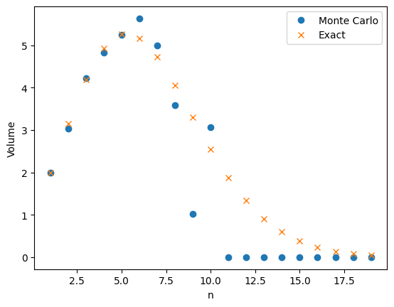
    The problem is that \(v_n\) is very small and the probability \(v_n/2^n\) is even smaller! For example when \(n = 10\), \(v_n/2^n \approx 0.0025\). This means that in our one thousand samples we only expect two or three occurrences of the event \(X_{m,1}^2 + \cdots + X_{m,n}^2 \le 1\). As a result our estimate has a high variance.

    The results get even worse as \(n\) increases. The probability \(v_n/2^n\) does to zero faster than exponentially. Even with a large value of \(M\), our estimate will be zero. Since \(v_n \neq 0\), the relative error in the approximation is 100%.

    Importance sampling

    Monte Carlo can still be used to approximate \(v_n\). Instead of using plain Monte Carlo, we can use a variance reduction technique called importance sampling (IS). Instead of sampling the points \(X_{m,1},\ldots, X_{m,n}\) from the uniform distribution on \([-1,1]\), we can instead sample the from some other distribution called a proposal distribution. The proposal distribution should be chosen so that that the event \(X_{m,1}^2 +\cdots +X_{m,n}^2 \le 1\) becomes more likely.

    In importance sampling, we need to correct for the fact that we are using a new distribution instead of the uniform distribution. Instead of the counting the number of times \(X_{m,1}^2+\cdots+X_{m,n}^2 \le 1\) , we give weights to each of samples and then add up the weights.

    If \(p\) is the density of the uniform distribution on \([-1,1]\) (the target distribution) and \(q\) is the density of the proposal distribution, then the IS Monte Carlo estimate of \(v_n\) is

    \(\displaystyle{\frac{1}{M}\sum_{m=1}^M Z_m \prod_{i=1}^n \frac{p(X_{m,i})}{q(X_{m,i})}},\)

    where as before \(Z_m\) is one if \(X_{m,1}^2+\cdots +X_{m,n}^2 \le 1\) and \(Z_m\) is zero otherwise. As long as \(q(x)=0\) implies \(p(x)=0\), the IS Monte Carlo estimate will be an unbiased estimate of \(v_n\). More importantly, a good choice of the proposal distribution \(q\) can drastically reduce the variance of the IS estimate compared to the plain Monte Carlo estimate.

    In this example, a good choice of proposal distribution is the normal distribution with mean \(0\) and variance \(1/n\). Under this proposal distribution, the expected value of \(X_{m,1}^2 +\cdots+ X_{m,n}^2\) is one and so the event \(X_{m,1}^2 + \cdots + X_{m,n}^2 \le 1\) is much more likely.

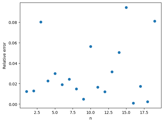
    Here are the IS Monte Carlo estimates with again \(M = 1,000\) and \(n\) ranging from \(1\) to \(20\). The results speak for themselves.

    The relative error is typically less than 10%. A big improvement over the 100% relative error of plain Monte Carlo.

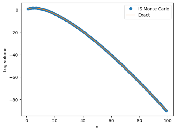
    The next plot shows a close agreement between \(v_n\) and the IS Monte Carlo approximation on the log scale with \(n\) going all the way up to \(100\).

    Notes

    1. There are exact formulas for \(v_n\) (available on Wikipedia). I used these to compare the approximations and compute relative errors. There are related problems where no formulas exist and Monte Carlo integration is one of the only ways to get an approximate answer.
    2. The post by John Cook also talks about why the central limit theorem can’t be used to approximate \(v_n\). I initially thought a technique called large deviations could be used to approximate \(v_n\) but again this does not directly apply. I was happy to discover that importance sampling worked so well!

    More sampling posts

  • Uniformly sampling orthogonal matrices

    An \(n \times n\) matrix \(M \in \mathbb{R}^{n \times n}\) is orthogonal if \(M^\top M = I\). The set of all \(n \times n\) orthogonal matrices is a compact group written as \(O_n\). The uniform distribution on \(O_n\) is called Haar measure. There are many ways to generate random matrices for Haar measure. One of which is based on the Gram-Schmidt algorithm.

    Proposition. Let \(X\) be a \(n \times n\) matrix such that each entry \(X_{ij}\) is an independent standard normal random variable. Let \(x_1,x_2,\ldots,x_n \in \mathbb{R}^n\) be the columns of \(X\) and let \(q_1,q_2,\ldots,q_n \in \mathbb{R}^n\) be the result of applying Gram-Schmidt to \(x_1,x_2,\ldots,x_n\). Then the matrix \(M=[q_1,q_2,\ldots,q_n] \in O_n\) is distributed according to Haar measure.

    Another way of stating the above proposition is that if \(X\) has i.i.d. standard normal entries, and \(Q,R\) is a QR-factorization of \(X\) calculated using Gram-Schmidt, then \(Q \in O_n\) is distributed according to Haar measure. However, most numerical libraries do not use Gram-Schmidt to calculate the QR-factorization of a matrix. This means that if you generate a random \(X\) and then use your computer’s QR-factorization function, then the result might not be Haar distributed as the plot below shows.

    The plot shows an estimate of the distribution of \(\sqrt{n}M_{11}\), the top-left entry of a matrix \(M\). When \(M\) is correctly sampled, the distribution is symmetric about 0. When \(M\) is incorrectly sampled the distribution is clearly biased towards negative numbers.

    Fortunately there is a fix described in [1]! We can first use any QR-factorization algorithm to produce \(Q,R\) with \(X=QR\). We then compute a diagonal matrix \(L\) with \(L_{ii} = \mathrm{Sign}(R_{ii})\). Then, the matrix \(M=QL\) is Haar distributed. The following python code thus samples a Haar distributed matrix in \(O_n\).

    import numpy as np

    def sample_M(n):
    M = np.random.randn(n, n)
    Q, R = np.linalg.qr(M)
    L = np.sign(np.diag(R))
    return Q*L[None,:]

    References

    [1] Mezzadri, Francesco. “How to generate random matrices from the classical compact groups.” arXiv preprint math-ph/0609050 (2006). https://arxiv.org/abs/math-ph/0609050

    I recently gave a talk at the Stanford student probability seminar on Haar distributed random matrices. My notes and many further references are available here.

  • Auxiliary variables sampler

    The auxiliary variables sampler is a general Markov chain Monte Carlo (MCMC) technique for sampling from probability distributions with unknown normalizing constants [1, Section 3.1]. Specifically, suppose we have \(n\) functions \(f_i : \mathcal{X} \to (0,\infty)\) and we want to sample from the probability distribution \(P(x) \propto \prod_{i=1}^n f_i(x).\) That is

    \(\displaystyle{ P(x) = \frac{1}{Z}\prod_{i=1}^n f_i(x)},\)

    where \(Z = \sum_{x \in \mathcal{X}} \prod_{i=1}^n f_i(x)\) is a normalizing constant. If the set \(\mathcal{X}\) is very large, then it may be difficult to compute \(Z\) or sample from \(P(x)\). To approximately sample from \(P(x)\) we can run an ergodic Markov chain with \(P(x)\) as a stationary distribution. Adding auxiliary variables is one way to create such a Markov chain. For each \(i \in \{1,\ldots,n\}\), we add a auxiliary variable \(U_i \ge 0\) such that

    \(\displaystyle{P(U \mid X) = \prod_{i=1}^n \mathrm{Unif}[0,f_i(X)]}.\)

    That is, conditional on \(X\), the auxiliary variables \(U_1,\ldots,U_n\) are independent and \(U_i\) is uniformly distributed on the interval \([0,f_i(X)]\). If \(X\) is distributed according to \(P\) and \(U_1,\ldots,U_n\) have the above auxiliary variable distribution, then

    \(\displaystyle{P(X,U) =P(X)P(U\mid X)\propto \prod_{i=1}^n f_i(X) \frac{1}{f_i(X)} I[U_i \le f(X_i)] = \prod_{i=1}^n I[U_i \le f(X_i)]}.\)

    This means that the joint distribution of \((X,U)\) is uniform on the set

    \(\widetilde{\mathcal{X}} = \{(x,u) \in \mathcal{X} \times (0,\infty)^n : u_i \le f(x_i) \text{ for all } i\}.\)

    Put another way, suppose we could jointly sample \((X,U)\) from the uniform distribution on \(\widetilde{\mathcal{X}}\). Then, the above calculation shows that if we discard \(U\) and only keep \(X\), then \(X\) will be sampled from our target distribution \(P\).

    The auxiliary variables sampler approximately samples from the uniform distribution on \(\widetilde{\mathcal{X}}\) is by using a Gibbs sampler. The Gibbs samplers alternates between sampling \(U’\) from \(P(U \mid X)\) and then sampling \(X’\) from \(P(X \mid U’)\). Since the joint distribution of \((X,U)\) is uniform on \(\widetilde{\mathcal{X}}\), the conditional distributions \(P(X \mid U)\) and \(P(U \mid X)\) are also uniform. The auxiliary variables sampler thus transitions from \(X\) to \(X’\) according to the two step process

    1. Independently sample \(U_i\) uniformly from \([0,f_i(X)]\).
    2. Sample \(X’\) uniformly from the set \(\{x \in \mathcal{X} : f_i(x) \ge u_i \text{ for all } i\}\).

    Since the auxiliary variables sampler is based on a Gibbs sampler, we know that the joint distribution of \((X,U)\) will converge to the uniform distribution on \(\mathcal{X}\). So when we discard \(U\), the distribution of \(X\) will converge to the target distribution \(P\)!

    Auxiliary variables in practice

    To perform step 2 of the auxiliary variables sampler we have to be able to sample uniformly from the sets

    \(\mathcal{X}_u = \{x \in \mathcal{X}:f_i(x) \ge u_i \text{ for all } i\}. \)

    Depending on the nature of the set \(\mathcal{X}\) and the functions \(f_i\), it might be difficult to do this. Fortunately, there are some notable examples where this step has been worked out. The very first example of auxiliary variables is the Swendsen-Wang algorithm for sampling from the Ising model [2]. In this model it is possible to sample uniformly from \(\mathcal{X}_u\). Another setting where we can sample exactly is when \(\mathcal{X}\) is the real numbers \(\mathcal{R}\) and each \(f_i\) is an increasing function of \(x\). This is explored in [3] where they apply auxiliary variables to sampling from Bayesian posteriors.

    There is an alternative to sampling exactly from the uniform distribution on \(\mathcal{X}_u\). Instead of sampling \(X’\) uniformly from \(\mathcal{X}_u\), we can run a Markov chain from the old \(X\) that has the uniform distribution as a stationary distribution. This approach leads to another special case of auxiliary variables which is called “slice sampling” [4].

    References

    [1] Andersen HC, Diaconis P. Hit and run as a unifying device. Journal de la societe francaise de statistique & revue de statistique appliquee. 2007;148(4):5-28. http://www.numdam.org/item/JSFS_2007__148_4_5_0/
    [2] Swendsen RH, Wang JS. Nonuniversal critical dynamics in Monte Carlo simulations. Physical review letters. 1987 Jan 12;58(2):86. https://journals.aps.org/prl/abstract/10.1103/PhysRevLett.58.86
    [3] Damlen P, Wakefield J, Walker S. Gibbs sampling for Bayesian non‐conjugate and hierarchical models by using auxiliary variables. Journal of the Royal Statistical Society: Series B (Statistical Methodology). 1999 Apr;61(2):331-44. https://rss.onlinelibrary.wiley.com/doi/abs/10.1111/1467-9868.00179
    [4] Neal RM. Slice sampling. The annals of statistics. 2003 Jun;31(3):705-67. https://projecteuclid.org/journals/annals-of-statistics/volume-31/issue-3/Slice-sampling/10.1214/aos/1056562461.full

  • Doing Calvin’s homework

    Growing up, my siblings and I would read a lot of Bill Watterson’s Calvin and Hobbes. I have fond memories of spending hours reading and re-reading our grandparents collection during the school holidays. The comic strip is witty, heartwarming and beautifully drawn.

    Recently, I came across this strip online

    Originally published Feb 5th, 1990 by Bill Watterson. All creative credit goes to Bill. You can read the rest of the story arc here: https://www.gocomics.com/calvinandhobbes/1990/02/05

    Seeing Calvin take this test took me back to those school holidays. I remember grabbing paper and a pencil to work out the answer (I also remember getting teased by those previously mentioned siblings). Reading the strip years later, I realized there’s a neat way to work out the answer without having to write much down. Here’s the question again,

    Jack and Joe leave their homes at the same time and drive toward each other. Jack drives at 60 mph, while Joe drives at 30 mph. They pass each other in 10 minutes.

    How far apart were Jack and Joe when they started?

    It can be hard to think about Jack and Joe traveling at different speeds. But we can simplify the problem by thinking from Joe’s perspective or frame of reference. From Joe’s frame of reference, he is staying perfectly still but Jack is zooming towards him at \(30+60=90\) mph. Jack reaches Joe in 10 minutes which is one sixth of an hour. This means that the initial distance between them must have been \(90 \times 1/6 = 15\) miles.

    It’s not as creative as Calvin’s private eye approach but at least Susie and I got the same answer.

    Originally published Feb 10th, 1990 by Bill Watterson. Again all creative credit goes to Bill. https://www.gocomics.com/calvinandhobbes/1990/02/10
  • Solving a system of equations vs inverting a matrix

    I used to have trouble understanding why inverting an \(n \times n\) matrix required the same order of operations as solving an \(n \times n\) system of linear equations. Specifically, if \(A\) is an \(n\times n\) invertible matrix and \(b\) is a length \(n\) vector, then computing \(A^{-1}\) and solving the equation \(Ax = b\) can both be done in \(O(n^3)\) floating point operations (flops). This surprised me because naively computing the columns of \(A^{-1}\) requires solving the \(n\) systems of equations

    \(Ax = e_1, Ax=e_2,\ldots, Ax = e_n,\)

    where \(e_1,e_2,\ldots, e_n\) are the standard basis vectors. I thought this would mean that calculating \(A^{-1}\) would require roughly \(n\) times as many flops as solving a single system of equations. It was only in a convex optimization lecture that I realized what was going on.

    To solve a single system of equations \(Ax = b\), we first compute a factorization of \(A\) such as the LU factorization. Computing this factorization takes \(O(n^3)\) flops but once we have it, we can use it solve any new system with \(O(n^2)\) flops. Now to solve \(Ax=e_1,Ax=e_2,\ldots,Ax=e_n\), we can simply factor \(A\) once and the perform \(n\) solves using the factorization each of which requires an addition \(O(n^2)\) flops. The total flop count is then \(O(n^3)+nO(n^2)=O(n^3)\). Inverting the matrix requires the same order of flops as a single solve!

    Of course, as John D Cook points out: you shouldn’t ever invert a matrix. Even if inverting and solving take the same order of flops, inverting is still more computational expensive and requires more memory.

    Related posts