Recent Posts

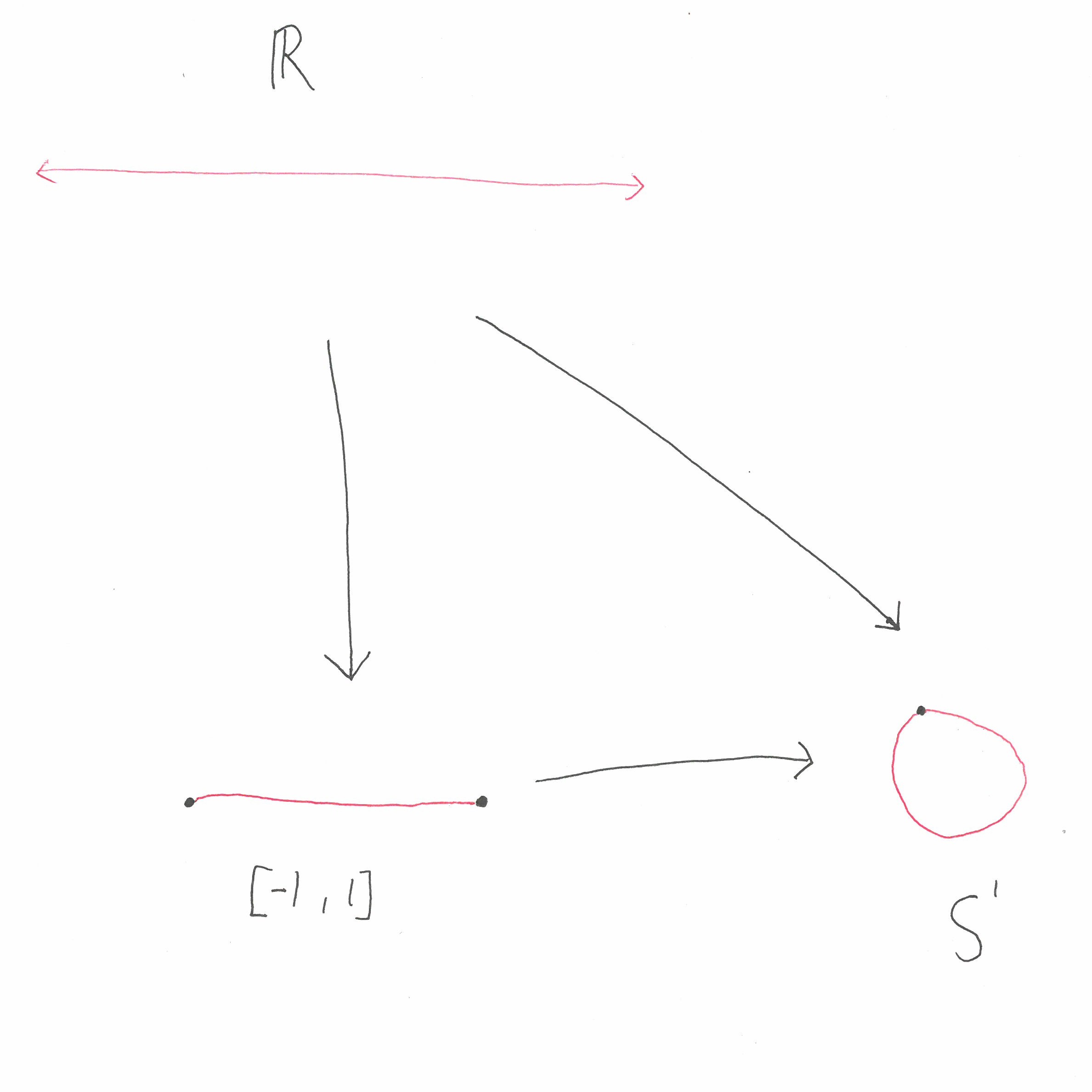
In the first blog post of this series we discussed two compactifications of \(\mathbb{R}\). We had the circle \(S^1\) and the interval \([-1,1]\). In the second post of this series we saw that there is a correspondence between compactifications of \(\mathbb{R}\) and sub algebras of \(C_b(\mathbb{R})\). In this blog post we will use this correspondence to uncover another compactification of \(\mathbb{R}\).

Since \(S^1\) is the one point compactification of \(\mathbb{R}\) we know that it corresponds to the subalgebra \(C_\infty(\mathbb{R})\). This can be seen by noting that a continuous function on \(S^1\) is equivalent to a continuous function, \(f\), on \(\mathbb{R}\) such that \(\lim_{x \to +\infty} f(x)\) and \(\lim_{x \to -\infty} f(x)\) both exist and are equal. On the other hand the compactification \([-1,1]\) corresponds to the space of functions \(f \in C_b(\mathbb{R})\) such that \(\lim_{x \to +\infty} f(x)\) and \(\lim_{x \to – \infty}f(x)\) both exist (but these limits need not be equal).

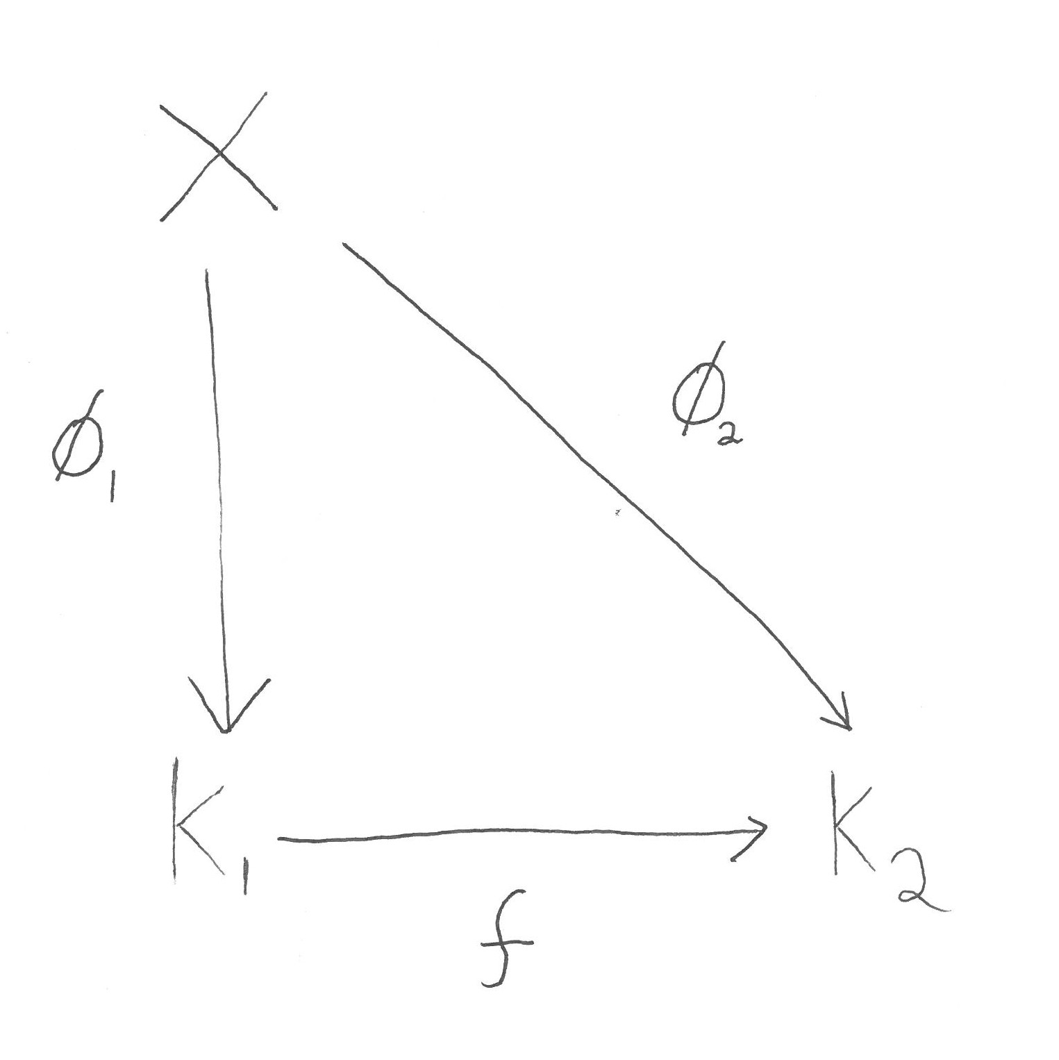
We can also play this game in reverse. We can start with an algebra \(A \subseteq C_b(\mathbb{R})\) and ask what compactification of \(\mathbb{R}\) it corresponds to. For example we may take \(A\) to be the following sub algebra

\(\{g+h \mid g,h \in C(\mathbb{R}), g(x+2\pi)=g(x) \text{ for all } x \in \mathbb{R} \text{ and } \lim_{x \to \pm \infty} h(x)=0 \}.\)

That is \(A\) contains precisely those functions in \(C_b(\mathbb{R})\) that are the perturbation of a \(2\pi\) periodic function by a function that vanishes at both \( \infty\) and \(– \infty\). Since any constant function is \(2 \pi\) periodic, we know that \(C_\infty(\mathbb{R})\) is contained in \(A\). Thus, as explained in the previous blog post, we know that \(\sigma(A)\) corresponds to a compactification of \(\mathbb{R}\).

Recall that \(\sigma(A)\) consists of all the non-zero continuous C*-homeomorphisms from \(A\) to \(\mathbb{C}\). The space \(\sigma(A)\) contains a copy o \(\mathbb{R}\) as a subspace. A point \(t \in \mathbb{R}\) corresponds to the homeomorphism \(\omega_t\) given by \(\omega_t(f)=f(t)\). There are also a circle’s worth of homeomorphisms \(\nu_p\) given by \(\nu_p(f) = \lim_{k \to \infty} f(2 \pi k+p)\) for \(p \in [0,2\pi)\). The homeomorphism \(\nu_p\) isolates the value of the \(2\pi\) periodic part of \(f\) at the point \(p\). This is because if \(f = g+h\) with \(g\) a \(2 \pi\) periodic function and \(h\) a function that vanishes at infinity. Then

\(\nu_p(f) = \lim\limits_{k \to \infty} (g(2 \pi k + p)+h(2 \pi k + p)) = g(p)+\lim\limits_{k \to \infty} h(2 \pi k + p) = g(p)\).

Thus we know that the topological space \(\sigma(A)\) is the union of a line and a circle. We now just need to work out the topology of how these to spaces are put together to make \(\sigma(A)\). We need to work out which points on the line are “close” to our points on the circle. Suppose we have a sequence of real numbers \((t_n)_{n \in \mathbb{N}}\) and a point \(p \in [0,2\pi)\) such that the following two conditions are satisfied. Firstly \(| t_n | \rightarrow \infty\) and secondly there exists a sequence of integers \((k_n)_{n \in \mathbb{N}}\) such that \(\lim\limits_{n \to \infty} (t_n – 2\pi k_n) = p\). Then we would have that \(\omega_{t_n}\) converges to \(\nu_p\) in \(\sigma(A)\).

Thus we know that the copy of \(\mathbb{R}\) in must spiral towards the copy of \(S^1\) in \(\sigma(A)\) and that this spiraling must happen as we approach either positive infinity or negative infinity. Thus we can realise \(\sigma(A)\) as the following subset of \(\mathbb{R}^3\) that looks a bit like Christmas tree decoration:

• 

• 

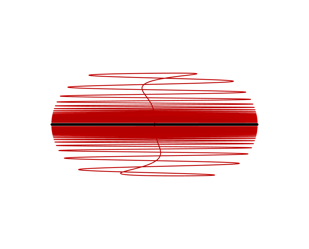
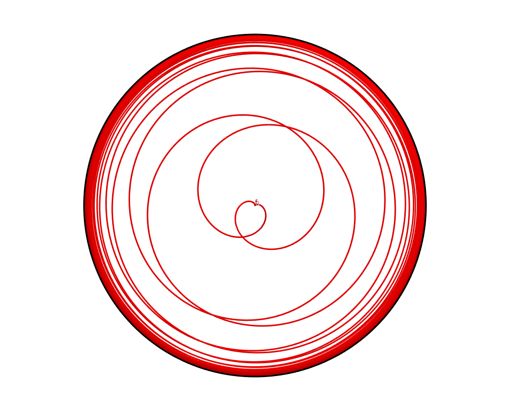
Here we have the black circle sitting in the x,y plane of \(\mathbb{R}^3\). The red line is a copy of \(\mathbb{R}\) that spirals towards the circle. Negative numbers sit below the circle and positive numbers sit above. On left is a sideways view of this space and on the right is the view from above. I made these images in geogebra. If you follow this link, you can see the equations that define the above space and move the space around.

This example shows just how complicated the Stone-Čech compactification \(\beta \mathbb{R}\) of \(\mathbb{R}\) must be. Our relatively simple algebra \(A\) gave this quite complicated compactification shown above. The Stone-Čech compactification surjects onto the above compactification and corresponds to the huge algebra of all bounded and continuous function from \(\mathbb{R}\) to \(\mathbb{C}\).

References

The Wikipedia page on the Stone-Čech compactification and these notes by Terrence Tao were where I first learned of the Stone-Čech compactification. I learnt about C*-algebras in a great course on operator algebras run by James Tenner at ANU. We used the textbook A Short Course on Spectral Theory by William Averson which has some exercises at the end of chapter 2 about the Stone-Čech compactification of \(\mathbb{R}\). The example of the algebra \(A \subseteq C_b(\mathbb{R})\) used in this blog post came from an assignment question set by James.

Parts one and two of this series can be found here.

This is the second post in a series about the Stone-Čech compactification. In the previous post we discussed compactifications and defined the Stone-Čech compactification. In this blog post we will show the existence of the Stone-Čech compactification of an arbitrary space. To do this we will use a surprising tool, C*-algebras. In the final blog post we take a closer look at what’s going on when our space is \(\mathbb{R}\).

The C*-algebra of operators on a Hilbert space

Before I define what a C*-algebra is, it is good to see a few examples of C*-algebras. If \(H\) is a Hilbert space over the complex numbers, then we define \(B(H)\) the space of bounded linear operators from \(H\) to \(H\). The space \(B(H)\) is a Banach space under the operator norm. The space \(B(H)\) is also a unital algebra since we can compose operators in \(B(H)\) and the identity operator acts as a unit. This composition satisfies the inequality \(\Vert ST \Vert \le \Vert S \Vert \Vert T \Vert \) for all \(S,T \in B(H)\). Thus \(B(H)\) is a Banach algebra. Finally we have an involution \(* : B(H) \rightarrow B(H)\) given by the adjoint. That is if \(T\) is a bounded operator on \(H\), then \(T^*\) is the unique bounded operator satisfying

\(\langle T h, g \rangle = \langle h, T^* g \rangle\),

for every \(h,g \in H\). This involution is conjugate linear and satisfies \((ST)^* = T^*S^*\) for all \(S, T \in B(H)\). This involution also satisfies the C*-property that \(\Vert T^*T\Vert = \Vert T \Vert^2\) for all \(T \in B(H)\).

The C*-algebra of continuous functions on a compact set

If \(K\) is a compact topological space, then the Banach space \(C(K)\) of continuous functions from \(K\) to \(\mathbb{C}\) is a unital Banach algebra. The norm on this space is the supremum norm

\(\Vert f \Vert = \sup_{x \in K} \vert f(x) \vert\)

and multiplication is defined pointwise. This algebra has a unit which is the function that is constantly one. This space also has an involution \(* : C(K) \rightarrow C(K)\) given by \(f^*(x) = \overline{f(x)}\). This involution is also conjugate linear and it satisfies \((fg)^* = f^*g^* = g^*f^*\) and the C*-property \(\Vert f^*f \Vert = \Vert f \Vert^2\).

Both \(B(H)\) and \(C(K)\) are examples of unital C*-algebras. We will define a unital C*-algebra to be a unital Banach algebra \(A\) with an involution \(* : A \rightarrow A\) such that

1. The involution is conjugate linear.
2. \((ab)^* = b^*a^*\) for all \(a, b \in A\).
3. \(\Vert a^*a \Vert = \Vert a \Vert^2\) for all \(a \in A\).

Our two examples \(B(H)\) and \(C(K)\) are different in one important way. The C*-algebra \(C(K)\) is commutative whereas in general \(B(H)\) is not. In some sense the C*-algebras \(C(K)\) are the only commutative unital C*-algebras. It is the precise statement of this fact that will let us define the Stone-Čech compactification of a space.

The Gelfand spectrum

If \(A\) is any unital C*-algebra we can define it’s Gelfand spectrum \(\sigma(A)\) to be the set of all continuous, non-zero C*-homomorphisms from \(A\) to \(\mathbb{C}\). That is every \(\omega \in \sigma(A)\) is a non-zero continuous linear functional from \(A\) to \(\mathbb{C}\) such that \( \omega (ab) = \omega (a) \omega (b)\) and \( \omega (a^*) = \overline{ \omega (a)}\). It can be shown that \(\sigma(A)\) is a weak*-closed subset of the unit ball in \(A’\), the dual of \(A\). Thus by the Banach-Alaoglu theorem, \(\sigma(A)\) is compact in the relative weak*-topology.

For example, take \(A = C(K)\) for some compact Hausdorff set \(K\). In this case we have a map from \(K\) to \(\sigma(C(K))\) given by \(p \mapsto \ \omega _p\) where \( \omega _p : C(K) \rightarrow \mathbb{C}\) is the evaluation map given by \( \omega _p(f) = f(p)\). This gives a continuous injection from \(K\) into \(\sigma(C(K))\). It turns out that this map is in fact also surjective and hence a homeomorphism between \(K\) and \(\sigma(C(K))\). Thus every continuous non-zero homeomorphism on \(C(K)\) is of the form \(\omega_p\) for some \(p \in K\). Thus we may simply regard \(\sigma(C(K))\) as being equal to \(K\).

The Gelfand spectrum \(\sigma(A)\) contains essentially all of the information about \(A\) when \(A\) is a commutative C*-algebra. This claim is made precise by the following theorem.

Theorem: If \(A\) is a unital commutative C*-algebra, then \(A\) is C*-isometric to \(C(\sigma(A))\), the space of continuous functions \(f : \sigma(A) \to \mathbb{C}\). This isomorphism is given by the map \(a\in A \mapsto f_a\) where \(f_a : \sigma(A) \rightarrow \mathbb{C}\) is given by \(f_a( \omega) = \omega (a)\) for all \(\omega \in \sigma(A)\).

This powerful theorem tells us that every unital commutative C*-algebra is of the form \(C(K)\) for some compact space \(K\). Furthermore this theorem tells us that we can take \(K\) to be the Gelfand spectrum of our C*-algebra.

The Gelfand spectrum and compactifications

We will now turn back to our original goal of constructing compactifications. If \(X\) is a locally compact Hausdorff space then we can define \(C_\infty(X)\) to be the space of continuous functions \(f : X \rightarrow \mathbb{C}\) that “have a limit at infinity”. By this we mean that for every \(f \in C_\infty(X)\) there exists a constant \(c \in \mathbb{C}\) such that for all \(\varepsilon > 0\), there exists a compact set \(K \subseteq X\) such that \(|f(x)-c| < \varepsilon\) for all \(x \in X \setminus K\). If we equip \(C_\infty(X)\) with the supremum norm and define \(f^*(x) = \overline{f(x)}\), then \(C_\infty(X)\) becomes a commutative unital C*-algebra under point-wise addition and multiplication.

We have a map from \(X\) to \(\sigma(C_\infty(X))\) given by evaluation. This map is still an homeomorphism onto its image but the map is not surjective if \(X\) is not compact. In the case when \(X\) is not compact, we have an extra element of \(\omega_\infty\) given by \(\omega_\infty(f) = \lim f\). Thus we have that \(\sigma(C_\infty(X)) \cong X \cup \{\omega_\infty\}\) and hence we have rediscovered the one-point compactification of \(X\).

A similar approach can be used to construct the Stone-Čech compactification. Rather than using the C*-algebra \(C_\infty(X)\), we will use the C*-algebra \(C_b(X)\) of all continuous and bounded functions from \(X\) to \(\mathbb{C}\). This is a C*-algebra under the supremum norm. We will show that the space \(\beta X := \sigma(C_b(X))\) satisfies the universal property of the Stone-Čech compactification. The map \(\phi : X \rightarrow \beta X\) is the same one given above. For any \(p \in X\), \(\phi(p) \in \beta X = \sigma(C_b(X))\) is defined to be the evaluation at \(p\) homomorphism \(\omega_p\). This map is a homeomorphism between \(X\) and an open dense subset of \(\beta X\). As in the case of the one point compactification, this map is not surjective. There are heaps of elements of \(\beta X \setminus \phi(X)\) as can be seen by the fact that \(\beta X\) surjects onto any other compactification of \(X\). However it is very hard to give an explicit definition of an element of \(\beta X \setminus X\).

We will now show that \(\beta X = \sigma(C_b(X))\) satisfies the universal property of the Stone-Čech compactification. Let \((K,\psi)\) be a compactification of \(X\). We wish to construct a morphism from \((\beta X,\phi)\) to \((K,\psi)\). That is we wish to find a map \(f : \beta X \rightarrow K\) such that \(f \circ \phi = \psi\). Note that such a map is automatically surjective as are all morphisms between compactifications. We can embed \(C(K)\) in \(C_b(X)\) by the map \(f \mapsto f \circ \psi\). Since \(\psi(X)\) is dense in \(K\), we have that this map is a C*-isometry from \(C(K)\) to its image in \(C_b(X)\). Above we argued that \(\sigma(C(K)) \cong K\). The compactification \((K,\psi)\) is in fact isomorphic to \((\sigma(C(K)), \widetilde {\psi})\) where \( \widetilde {\psi}(p)=\omega_{\psi(p)}\). Thus we will construct our morphism from \((\beta X, \phi)\) to \((\sigma(C(K)), \widetilde {\psi})\).

Now elements of \(\beta X \) are homeomorphism on \(C_b(X)\) and elements of \(\sigma(C(K))\) are homeomorphism on \(C(K)\). Since we can think of \(C(K)\) as being a subspace of \(C_b(K)\) we can define the map \(f : \beta X \rightarrow \sigma(C(K))\) to be restriction to \(C(K)\). That is \(f(\omega) = \omega_{\mid C(K)}\). Note that since \(C(K)\) contains the unit of \(C_b(X)\), the above map is well defined (in particular \(\omega \neq 0\) implies \(\omega_{\mid C(K)} \neq 0\)). One can check that the relation \(f \circ \phi = \widetilde{\psi}\) does indeed hold since both \(\phi\) and \(\widetilde{\psi}\) correspond to point evaluation. Thus we have realised the Stone-Čech compactification of \(X\) as the Gelfand spectrum of \(C_b(X)\).

The above argument can be modified to give a correspondence between compactifications of \(X\) and sub C*-algebras of \(C_b(X)\) that contain \(C_\infty(X)\). This correspondence is given by sending the sub C*-algebra \(A\) to \(\sigma(A)\) and the point evaluation map. This correspondence is order reversing in the sense that if we have \(A_1 \subseteq A_2\) for two sub C*-algebras, then we have a morphism from \(\sigma(A_2)\) to \(\sigma(A_1)\).

In the final blog post of the series we will further explore this correspondence between compactifications and subalgebras in the case when \(X = \mathbb{R}\). Part one of this series can be found here.

Mathematics is full of surprising connections between two seemingly unrelated topics. It’s one of the things I like most about maths. Over the next few blog posts I hope to explain one such connection which I’ve been thinking about a lot recently.

The Stone-Čech compactification connects the study of C*-algebras with topology. This first blog post will set the scene by explaining the topological notion of a compactification. In the next blog post, I’ll define and discuss C*-algebras and we’ll see how they can be used to study compactifications. In the final post we will look at a particular example.

Compactifications

Let \(X\) be a locally compact Hausdorff space. A compactification of \(X\) is a compact Hausdorff space \(K\) and a continuous function \(\phi : X \rightarrow K\) such that \(\phi\) is a homeomorphism between \(X\) and \(\phi(X)\) and \(\phi(X)\) is an open, dense subset of \(K\). Thus a compactification is a way of nicely embedding the space \(X\) into a compact space \(K\).

For example if \(X\) is the real line \(\mathbb{R}\), then the circle \(S^1\) and the stereographic projection is a compactification of \(X\). In this case the image of \(X\) is all of the circle apart from one point. Since the circle is compact, this is indeed a compactification. This is an example of a one-point compactification. An idea which we will return to later.

Comparing Compactifications

A space \(X\) will in general have many compactifications and we would like to compare these different compactifications. Suppose that \((K_1,\phi_1)\) and \((K_2, \phi_2)\) are two compactifications. Then a morphism from \((K_1,\phi_1)\) to \((K_2,\phi_2)\) is a continuous map \(f : K_1 \rightarrow K_2\) such that \(\phi_2 = f \circ \phi_1\). That is, the below diagram commutes:

Hence we have a morphism from \((K_1,\phi_1)\) to \((K_2,\phi_2)\) precisely when the embedding \(\phi_2 : X \rightarrow K_2\) extends to a map \(f : K_1 \rightarrow K_2\). Since \(\phi_1(X)\) is dense in \(K_1\), if such a function \(f\) exists, it is unique.

Note that the map \(f \) must be surjective since \(\phi_2(X)\) is dense in \(K_2\) and \(g(K_1)\) is a closed set containing \(\phi_2(X)\). We can think of the compactification \((K_1,\phi_1)\) as being “bigger” or “more general” than the compactification \((K_2, \phi_2)\) as \(f\) is a surjection onto \(K_2\). More formally we will say that \((K_1,\phi_1)\) is finer than \((K_2, \phi _2)\) and equivalently that \((K_2, \phi _2)\) is coarser than \((K_1, \phi _1)\) whenever there is a morphism from \((K_1, \phi_1)\) to \((K_2,\phi_2)\). Note that the composition of two morphism of compactifications is again a morphism of compactifications. Thus we can talk about the category of compactifications of a space. The compactifications \((K_1, \phi _1)\) and \((K_2, \phi _2)\) are isomorphic if there exists a morphism \(g\) between \((K_1, \phi _1)\) and \((K_2, \phi _2)\) such that \(g\) is a homeomorphism between \(K_1\) and \(K_2\).

For example again let \(X = \mathbb{R}\). Then the closed interval \([-1,1]\) is again a compactification of \(\mathbb{R}\) with the map \((x,y) \mapsto \frac{x}{1+|x|}\) which maps \(\mathbb{R}\) onto the open interval \((-1,1)\). We can then create a morphism from \([-1,1]\) to the circle by sending the endpoints of \([-1,1]\) to the top of the circle and sending the interior of \([-1,1]\) to the rest of the circle. We can perform this map in such a way that the following diagram commutes:

Thus we have a morphism from the compactification \([-1,1]\) to the compactification \(S^1\). Thus the compactification \([-1,1]\) is finer than the compactification \(S^1\).

Now that we have a way of comparing compactifications of \(X\) we can ask about the existence of extremal compactifications of \(X\). Does there exists a compactification of \(X\) that is the coarser than any other compactification? Or one which is finer than any other? From a category-theory perspective, we are interested in the existence of terminal and initial objects in the category of compactifications of \(X\). We will first show the existence of a coarsest or “least general” compactification.

The one point compactification

A coarsest compactification would be a terminal object in the category of compactifications. That is a compactification \((\alpha X, i)\) with the property that for all compactification \((K, \phi)\) there is a unique extension \(g : K \rightarrow \alpha X\) of \(i : X \rightarrow \alpha X\). If such a coarsest compactification exists, then it is unique up to isomorphism. Thus we can safely refer to the coarsest compactification.

The one point compactification of \(X\) is constructed by adding a single point denoted by \(\infty\) to \(X\). It is defined to be the set \(\alpha X = X \sqcup \{ \infty\}\) with the topology given by the collection of open sets in \(X\) and sets of the form \(\alpha X \setminus K\) for \(K \subseteq X\) a compact subset. The map \(i : X \rightarrow \alpha X\) is given by simply including \(X\) into \(\alpha X = X \sqcup \{\infty\}\).

The one point compactification is the coarsest compactification of \(X\). Let \((K,\phi)\) be another compactification of \(X\). Then the map \(g : K \rightarrow \alpha X\) given by

\(g(y) = \begin{cases} i(\phi^{-1}(y)) & \text{if } y \in \phi(X),\\ \infty & \text{if } y \notin \phi(X), \end{cases}\)

is the unique morphism from \((K,f)\) to \((\alpha X, i)\).

The Stone-Čech compactification

A Stone-Čech compactification of \(X\) is a compactification \((\beta X,j)\) which is the finest compactification of \(X\). That is \((\beta X,j)\) is an initial object in the category of a compactifications of \(X\) and so for every compactification \((K,f)\) there exists a unique morphism from \((\beta X,j)\) to \((K,f)\). Thus any embedding \(f : X \rightarrow K\), has a unique extension \(g : \beta X \rightarrow K\). As with coarest compactification of \(X\), the Stone-Čech compactification of \(X\) is unique up to isomorphism and thus we will talk of the Stone-Čech compactification.

Unlike the one point compactification of \(X\), there is no simple description of \(\beta X\) even when \(X\) is a very simple space such as \(\mathbb{N}\) or \(\mathbb{R}\). To show the existence of a Stone-Čech compactification of any space \(X\) we will need to make a detour and develop some tools from the study of C*-algebras which will be the topic of the next blog post.