Like my previous post, this blog is also motivated by a comment by Professor Persi Diaconis in his recent Stanford probability seminar. The seminar was about a way of “collapsing” a random walk on a group to a random walk on the set of double cosets. In this post, I’ll first define double cosets and then go over the example Professor Diaconis used to make us probabilists and statisticians more comfortable with all the group theory he was discussing.
Double cosets
Let \(G\) be a group and let \(H\) and \(K\) be two subgroups of \(G\). For each \(g \in G\), the \((H,K)\)-double coset containing \(g\) is defined to be the set
\(HgK = \{hgk : h \in H, k \in K\}\)
To simplify notation, we will simply write double coset instead of \((H,K)\)-double coset. The double coset of \(g\) can also be defined as the equivalence class of \(g\) under the relation
\(g \sim g’ \Longleftrightarrow g’ = hgk\) for some \(h \in H\) and \(g \in G\)
Like regular cosets, the above relation is indeed an equivalence relation. Thus, the group \(G\) can be written as a disjoint union of double cosets. The set of all double cosets of \(G\) is denoted by \(H\backslash G / K\). That is,
\(H\backslash G /K = \{HgK : g \in G\}\)
Note that if we take \(H = \{e\}\), the trivial subgroup, then the double cosets are simply the left cosets of \(K\), \(G / K\). Likewise if \(K = \{e\}\), then the double cosets are the right cosets of \(H\), \(H \backslash G\). Thus, double cosets generalise both left and right cosets.
Double cosets in \(S_n\)
Fix a natural number \(n > 0\). A partition of \(n\) is a finite sequence \(a = (a_1,a_2,\ldots, a_I)\) such that \(a_1,a_2,\ldots, a_I \in \mathbb{N}\), \(a_1 \ge a_2 \ge \ldots a_I > 0\) and \(\sum_{i=1}^I a_i = n\). For each partition of \(n\), \(a\), we can form a subgroup \(S_a\) of the symmetric group \(S_n\). The subgroup \(S_a\) contains all permutations \(\sigma \in S_n\) such that \(\sigma\) fixes the sets \(A_1 = \{1,\ldots, a_1\}, A_2 = \{a_1+1,\ldots, a_1 + a_2\},\ldots, A_I = \{n – a_I +1,\ldots, n\}\). Meaning that \(\sigma(A_i) = A_i\) for all \(1 \le i \le I\). Thus, a permutation \(\sigma \in S_a\) must individually permute the elements of \(A_1\), the elements of \(A_2\) and so on. This means that, in a natural way,
\(S_a \cong S_{a_1} \times S_{a_2} \times \ldots \times S_{a_I}\)
If we have two partitions \(a = (a_1,a_2,\ldots, a_I)\) and \(b = (b_1,b_2,\ldots,b_J)\), then we can form two subgroups \(H = S_a\) and \(K = S_b\) and consider the double cosets \(H \backslash G / K = S_a \backslash S_n / S_b\). The claim made in the seminar was that the double cosets are in one-to-one correspondence with \(I \times J\) contingency tables with row sums equal to \(a\) and column sums equal to \(b\). Before we explain this correspondence and properly define contingency tables, let’s first consider the cases when either \(H\) or \(K\) is the trivial subgroup.
Left cosets in \(S_n\)
Note that if \(a = (1,1,\ldots,1)\), then \(S_a\) is the trivial subgroup and, as noted above, \(S_a \backslash S_n / S_b\) is simply equal to \(S_n / S_b\). We will see that the cosets in \(S_n/S_b\) can be described by forgetting something about the permutations in \(S_n\).
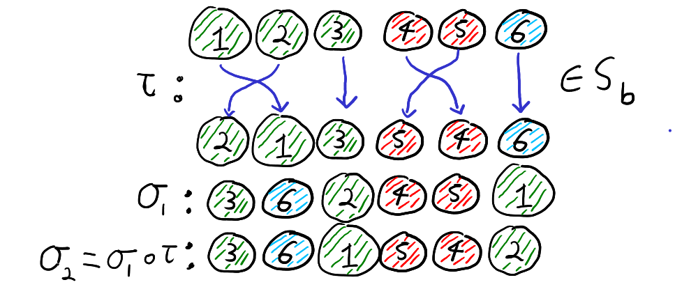
We can think of the permutations in \(S_n\) as all the ways of drawing without replacement \(n\) balls labelled \(1,2,\ldots, n\). We can think of the partition \(b = (b_1,b_2,\ldots,b_J)\) as a colouring of the \(n\) balls by \(J\) colours. We colour balls \(1,2,\ldots, b_1\) by the first colour \(c_1\), then we colour \(b_1+1,b_1+2,\ldots, b_1+b_2\) the second colour \(c_2\) and so on until we colour \(n-b_J+1, n-b_J+2,\ldots, n\) the final colour \(c_J\). Below is an example when \(n\) is equal to 6 and \(b = (3,2,1)\).

Note that a permutation \(\sigma \in S_n\) is in \(S_b\) if and only if we draw the balls by colour groups, i.e. we first draw all the balls with colour \(c_1\), then we draw all the balls with colour \(c_2\) and so on. Thus, continuing with the previous example, the permutation \(\sigma_1\) below is in \(S_b\) but \(\sigma_2\) is not in \(S_b\).

It turns out that we can think of the cosets in \(S_n \setminus S_b\) as what happens when we “forget” the labels \(1,2,\ldots,n\) and only remember the colours of the balls. By “forgetting” the labels we mean only paying attention to the list of colours. That is for all \(\sigma_1,\sigma_2 \in S_n\), \(\sigma_1 S_b = \sigma_2 S_b\) if and only if the list of colours from the draw \(\sigma_1\) is the same as the list of colours from the draw \(\sigma_2\). Thus, the below two permutations define the same coset of \(S_b\)

To see why this is true, note that \(\sigma_1 S_b = \sigma_2 S_b\) if and only if \(\sigma_2 = \sigma_1 \circ \tau\) for some \(\tau \in S_b\). Furthermore, \(\tau \in S_b\) if and only if \(\tau\) maps each colour group to itself. Recall that function composition is read right to left. Thus, the equation \(\sigma_2 = \sigma_1 \circ \tau\) means that if we first relabel the balls according to \(\tau\) and then draw the balls according to \(\sigma_1\), then we get the result as just drawing by \(\sigma_2\). That is, \(\sigma_2 = \sigma_1 \circ \tau\) for some \(\tau \in S_b\) if and only if drawing by \(\sigma_2\) is the same as first relabelling the balls within each colour group and then drawing the balls according to \(\sigma_1\). Thus, \(\sigma_1 S_b = \sigma_2 S_b\), if and only if when we forget the labels of the balls and only look at the colours, \(\sigma_1\) and \(\sigma_2\) give the same list of colours. This is illustrated with our running example below.

Right cosets of \(S_n\)
Typically, the subgroup \(S_a\) is not a normal subgroup of \(S_n\). This means that the right coset \(S_a \sigma\) will not equal the left coset \(\sigma S_a\). Thus, colouring the balls and forgetting the labelling won’t describe the right cosets \(S_a \backslash S_n\). We’ll see that a different type of forgetting can be used to describe \(S_a \backslash S_n = \{S_a\sigma : \sigma \in S_n\}\).
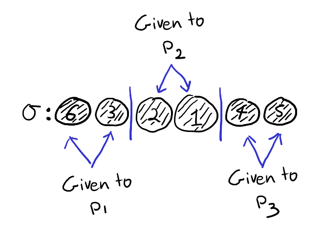
Fix a partition \(a = (a_1,a_2,\ldots,a_I)\) and now, instead of considering \(I\) colours, think of \(I\) different people \(p_1,p_2,\ldots,p_I\). As before, a permutation \(\sigma \in S_n\) can be thought of drawing \(n\) balls labelled \(1,\ldots,n\) without replacement. We can imagine giving the first \(a_1\) balls drawn to person \(p_1\), then giving the next \(a_2\) balls to the person \(p_2\) and so on until we give the last \(a_I\) balls to person \(p_I\). An example with \(n = 6\) and \(a = (2,2,2)\) is drawn below.

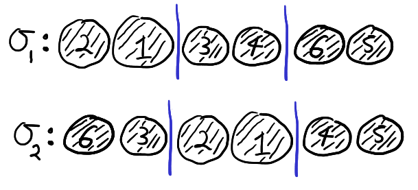
Note that \(\sigma \in S_a\) if and only if person \(p_i\) receives the balls with labels \(\sum_{k=0}^{i-1}a_k+1,\sum_{k=0}^{i-1}a_k+2,\ldots, \sum_{k=0}^i a_k\) in any order. Thus, in the below example \(\sigma_1 \in S_a\) but \(\sigma_2 \notin S_a\).

It turns out the cosets \(S_a \backslash S_n\) are exactly determined by “forgetting” the order in which each person \(p_i\) received their balls and only remembering which balls they received. Thus, the two permutation below belong to the same coset in \(S_a \backslash S_n\).

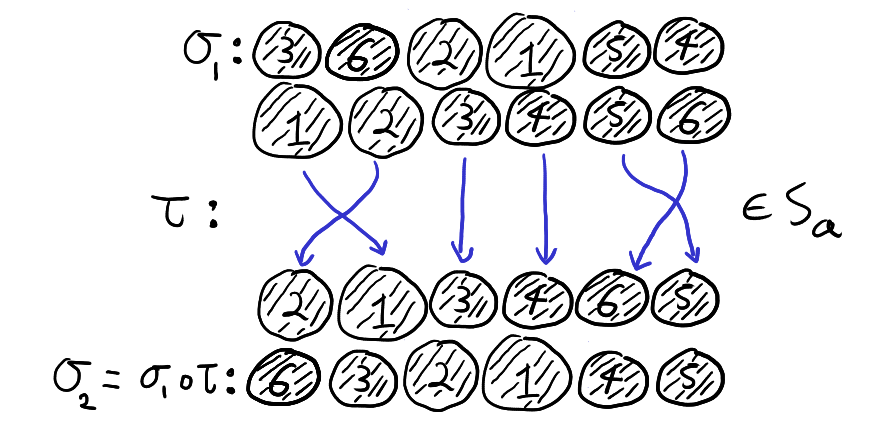
To see why this is true in general, consider two permutations \(\sigma_1,\sigma_2\). The permutations \(\sigma_1,\sigma_2\) result in each person \(p_i\) receiving the same balls if and only if after \(\sigma_1\) we can apply a permutation \(\tau\) that fixes each subset \(A_i = \left\{\sum_{k=0}^{i-1}a_k+1,\ldots, \sum_{k=0}^i a_k\right\}\) and get \(\sigma_2\). That is, \(\sigma_1\) and \(\sigma_2\) result in each person \(p_i\) receiving the same balls if and only if \(\sigma_2 = \tau \circ \sigma_1\) for some \(\tau \in S_a\). Thus, \(\sigma_1,\sigma_2\) are the same after forgetting the order in which each person received their balls if and only if \(S_a \sigma_1 = S_a \sigma_2\). This is illustrated below,

We can thus see why \(S_a \backslash S_n \neq S_n / S_a\). A left coset \(\sigma S_a\) correspond to pre-composing \(\sigma\) with elements of \(S_a\) and a right cosets \(S_a\sigma\) correspond to post-composing \(\sigma\) with elements of \(S_a\).
Contingency tables
With the last two sections under our belts, describing the double cosets \(S_a \backslash S_n / S_b\) is straight forward. We simply have to combine our two types of forgetting. That is, we first colour the \(n\) balls with \(J\) colours according to \(b = (b_1,b_2,\ldots,b_J)\). We then draw the balls without replace and give the balls to \(I\) different people according \(a = (a_1,a_2,\ldots,a_I)\). We then forget both the original labels and the order in which each person received their balls. That is, we only remember the number of balls of each colour each person receives. Describing the double cosets by “double forgetting” is illustrated below with \(a = (2,2,2)\) and \(b = (3,2,1)\).

The proof that double forgetting does indeed describe the double cosets is simply a combination of the two arguments given above. After double forgetting, the number of balls given to each person can be recorded in an \(I \times J\) table. The \(N_{ij}\) entry of the table is simply the number of balls person \(p_i\) receives of colour \(c_j\). Two permutations are the same after double forgetting if and only if they produce the same table. For example, \(\sigma_1\) and \(\sigma_2\) above both produce the following table
| Green (\(c_1\)) | Red (\(c_2\)) | Blue (\(c_3\)) | Total | |
| Person \(p_1\) | 1 | 0 | 1 | 2 |
| Person \(p_2\) | 1 | 1 | 0 | 2 |
| Person \(p_3\) | 1 | 1 | 0 | 2 |
| Total | 3 | 2 | 1 | 6 |
By the definition of how the balls are coloured and distributed to each person we must have for all \(1 \le i \le I\) and \(1 \le j \le J\)
\(\sum_{j=1}^J N_{ij} = a_i \) and \(\sum_{i=1}^I N_{ij} = b_j\)
An \(I \times J\) table with entries \(N_{ij} \in \{0,1,2,\ldots\}\) satisfying the above conditions is called a contingency table. Given such a contingency table with entries \(N_{ij}\) where the rows sum to \(a\) and the columns sum to \(b\), there always exists at least one permutation \(\sigma\) such that \(N_{ij}\) is the number of balls received by person \(p_i\) of colour \(c_i\). We have already seen that two permutations produce the same table if and only if they are in the same double coset. Thus, the double cosets \(S_a \backslash S_n /S_b\) are in one-to-one correspondence with such contingency tables.
The hypergeometric distribution
I would like to end this blog post with a little bit of probability and relate the contingency tables above to the hyper geometric distribution. If \(a = (m, n-m)\) for some \(m \in \{0,1,\ldots,n\}\), then the contingency tables described above have two rows and are determined by the values \(N_{11}, N_{12},\ldots, N_{1J}\) in the first row. The numbers \(N_{1j}\) are the number of balls of colour \(c_j\) the first person receives. Since the balls are drawn without replacement, this means that if we put the uniform distribution on \(S_n\), then the vector \(Y=(N_{11}, N_{12},\ldots, N_{1J})\) follows the multivariate hypergeometric distribution. Thus, if we have a random walk on \(S_n\) that quickly converges to the uniform distribution on \(S_n\), then we could use the double cosets to get a random walk that converges to the multivariate hypergeometric distribution (although there are smarter ways to do such sampling).
2 thoughts on “Double cosets and contingency tables”