Category: Uncategorized

  • Double cosets and contingency tables

    Like my previous post, this blog is also motivated by a comment by Professor Persi Diaconis in his recent Stanford probability seminar. The seminar was about a way of “collapsing” a random walk on a group to a random walk on the set of double cosets. In this post, I’ll first define double cosets and then go over the example Professor Diaconis used to make us probabilists and statisticians more comfortable with all the group theory he was discussing.

    Double cosets

    Let \(G\) be a group and let \(H\) and \(K\) be two subgroups of \(G\). For each \(g \in G\), the \((H,K)\)-double coset containing \(g\) is defined to be the set

    \(HgK = \{hgk : h \in H, k \in K\}\)

    To simplify notation, we will simply write double coset instead of \((H,K)\)-double coset. The double coset of \(g\) can also be defined as the equivalence class of \(g\) under the relation

    \(g \sim g’ \Longleftrightarrow g’ = hgk\) for some \(h \in H\) and \(g \in G\)

    Like regular cosets, the above relation is indeed an equivalence relation. Thus, the group \(G\) can be written as a disjoint union of double cosets. The set of all double cosets of \(G\) is denoted by \(H\backslash G / K\). That is,

    \(H\backslash G /K = \{HgK : g \in G\}\)

    Note that if we take \(H = \{e\}\), the trivial subgroup, then the double cosets are simply the left cosets of \(K\), \(G / K\). Likewise if \(K = \{e\}\), then the double cosets are the right cosets of \(H\), \(H \backslash G\). Thus, double cosets generalise both left and right cosets.

    Double cosets in \(S_n\)

    Fix a natural number \(n > 0\). A partition of \(n\) is a finite sequence \(a = (a_1,a_2,\ldots, a_I)\) such that \(a_1,a_2,\ldots, a_I \in \mathbb{N}\), \(a_1 \ge a_2 \ge \ldots a_I > 0\) and \(\sum_{i=1}^I a_i = n\). For each partition of \(n\), \(a\), we can form a subgroup \(S_a\) of the symmetric group \(S_n\). The subgroup \(S_a\) contains all permutations \(\sigma \in S_n\) such that \(\sigma\) fixes the sets \(A_1 = \{1,\ldots, a_1\}, A_2 = \{a_1+1,\ldots, a_1 + a_2\},\ldots, A_I = \{n – a_I +1,\ldots, n\}\). Meaning that \(\sigma(A_i) = A_i\) for all \(1 \le i \le I\). Thus, a permutation \(\sigma \in S_a\) must individually permute the elements of \(A_1\), the elements of \(A_2\) and so on. This means that, in a natural way,

    \(S_a \cong S_{a_1} \times S_{a_2} \times \ldots \times S_{a_I}\)

    If we have two partitions \(a = (a_1,a_2,\ldots, a_I)\) and \(b = (b_1,b_2,\ldots,b_J)\), then we can form two subgroups \(H = S_a\) and \(K = S_b\) and consider the double cosets \(H \backslash G / K = S_a \backslash S_n / S_b\). The claim made in the seminar was that the double cosets are in one-to-one correspondence with \(I \times J\) contingency tables with row sums equal to \(a\) and column sums equal to \(b\). Before we explain this correspondence and properly define contingency tables, let’s first consider the cases when either \(H\) or \(K\) is the trivial subgroup.

    Left cosets in \(S_n\)

    Note that if \(a = (1,1,\ldots,1)\), then \(S_a\) is the trivial subgroup and, as noted above, \(S_a \backslash S_n / S_b\) is simply equal to \(S_n / S_b\). We will see that the cosets in \(S_n/S_b\) can be described by forgetting something about the permutations in \(S_n\).

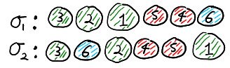
    We can think of the permutations in \(S_n\) as all the ways of drawing without replacement \(n\) balls labelled \(1,2,\ldots, n\). We can think of the partition \(b = (b_1,b_2,\ldots,b_J)\) as a colouring of the \(n\) balls by \(J\) colours. We colour balls \(1,2,\ldots, b_1\) by the first colour \(c_1\), then we colour \(b_1+1,b_1+2,\ldots, b_1+b_2\) the second colour \(c_2\) and so on until we colour \(n-b_J+1, n-b_J+2,\ldots, n\) the final colour \(c_J\). Below is an example when \(n\) is equal to 6 and \(b = (3,2,1)\).

    The first three balls are coloured green, the next two are coloured red and the last ball is coloured blue.

    Note that a permutation \(\sigma \in S_n\) is in \(S_b\) if and only if we draw the balls by colour groups, i.e. we first draw all the balls with colour \(c_1\), then we draw all the balls with colour \(c_2\) and so on. Thus, continuing with the previous example, the permutation \(\sigma_1\) below is in \(S_b\) but \(\sigma_2\) is not in \(S_b\).

    The permutation \(\sigma_1\) is in \(S_b\) because the colours are in their original order but \(\sigma_1\) is not in \(S_b\) because the colours are rearranged.

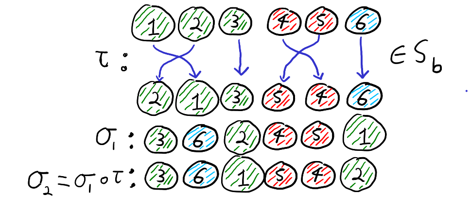
    It turns out that we can think of the cosets in \(S_n \setminus S_b\) as what happens when we “forget” the labels \(1,2,\ldots,n\) and only remember the colours of the balls. By “forgetting” the labels we mean only paying attention to the list of colours. That is for all \(\sigma_1,\sigma_2 \in S_n\), \(\sigma_1 S_b = \sigma_2 S_b\) if and only if the list of colours from the draw \(\sigma_1\) is the same as the list of colours from the draw \(\sigma_2\). Thus, the below two permutations define the same coset of \(S_b\)

    When we forget the labels and only remember the colours, the permutations \(\sigma_1\) and \(\sigma_2\) look the same and thus are in the same left coset of \(S_b\).

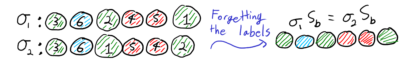
    To see why this is true, note that \(\sigma_1 S_b = \sigma_2 S_b\) if and only if \(\sigma_2 = \sigma_1 \circ \tau\) for some \(\tau \in S_b\). Furthermore, \(\tau \in S_b\) if and only if \(\tau\) maps each colour group to itself. Recall that function composition is read right to left. Thus, the equation \(\sigma_2 = \sigma_1 \circ \tau\) means that if we first relabel the balls according to \(\tau\) and then draw the balls according to \(\sigma_1\), then we get the result as just drawing by \(\sigma_2\). That is, \(\sigma_2 = \sigma_1 \circ \tau\) for some \(\tau \in S_b\) if and only if drawing by \(\sigma_2\) is the same as first relabelling the balls within each colour group and then drawing the balls according to \(\sigma_1\). Thus, \(\sigma_1 S_b = \sigma_2 S_b\), if and only if when we forget the labels of the balls and only look at the colours, \(\sigma_1\) and \(\sigma_2\) give the same list of colours. This is illustrated with our running example below.

    If we permute the balls according to \(\tau \in S_b\) and the draw according to \(\sigma_1\), then the resulting draw is the same as if we had not permuted and drawn according to \(\sigma_2\). That is, \(\sigma_2 = \sigma_1 \circ \tau\).

    Right cosets of \(S_n\)

    Typically, the subgroup \(S_a\) is not a normal subgroup of \(S_n\). This means that the right coset \(S_a \sigma\) will not equal the left coset \(\sigma S_a\). Thus, colouring the balls and forgetting the labelling won’t describe the right cosets \(S_a \backslash S_n\). We’ll see that a different type of forgetting can be used to describe \(S_a \backslash S_n = \{S_a\sigma : \sigma \in S_n\}\).

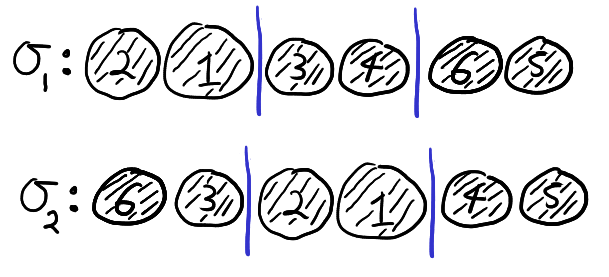
    Fix a partition \(a = (a_1,a_2,\ldots,a_I)\) and now, instead of considering \(I\) colours, think of \(I\) different people \(p_1,p_2,\ldots,p_I\). As before, a permutation \(\sigma \in S_n\) can be thought of drawing \(n\) balls labelled \(1,\ldots,n\) without replacement. We can imagine giving the first \(a_1\) balls drawn to person \(p_1\), then giving the next \(a_2\) balls to the person \(p_2\) and so on until we give the last \(a_I\) balls to person \(p_I\). An example with \(n = 6\) and \(a = (2,2,2)\) is drawn below.

    Person \(p_1\) receives the ball labelled by 6 followed by the ball labelled 3, person \(p_2\) receives ball 2 and then ball 1 and finally person \(p_3\) receives ball 4 followed by ball 5.

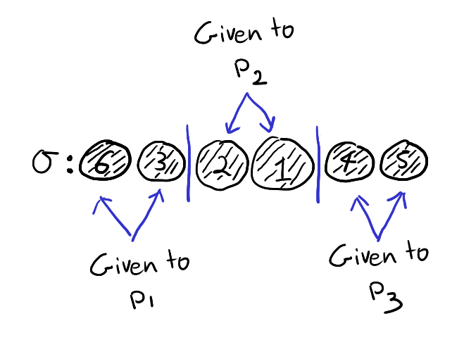
    Note that \(\sigma \in S_a\) if and only if person \(p_i\) receives the balls with labels \(\sum_{k=0}^{i-1}a_k+1,\sum_{k=0}^{i-1}a_k+2,\ldots, \sum_{k=0}^i a_k\) in any order. Thus, in the below example \(\sigma_1 \in S_a\) but \(\sigma_2 \notin S_a\).

    When the balls are drawn according to \(\sigma_1\), person \(p_i\) receives the balls with labels \(2i-1\) and \(2i\), and thus \(\sigma_1 \in S_a\). On the other hand, if the balls are drawn according to \(\sigma_2\), the people receive different balls and thus \(\sigma_2 \notin S_a\).

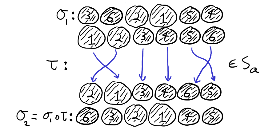
    It turns out the cosets \(S_a \backslash S_n\) are exactly determined by “forgetting” the order in which each person \(p_i\) received their balls and only remembering which balls they received. Thus, the two permutation below belong to the same coset in \(S_a \backslash S_n\).

    When we forget the order in which each person receive their balls, the permutations \(\sigma_1\) and \(\sigma_2\) become the same and thus \(S_a \sigma_1 = S_a \sigma_2\). Note that if we coloured the balls according to the permutation \(a = (a_1,\ldots,a_I)\), then we could see that \(\sigma_1 S_a \neq \sigma_2 S_a\).

    To see why this is true in general, consider two permutations \(\sigma_1,\sigma_2\). The permutations \(\sigma_1,\sigma_2\) result in each person \(p_i\) receiving the same balls if and only if after \(\sigma_1\) we can apply a permutation \(\tau\) that fixes each subset \(A_i = \left\{\sum_{k=0}^{i-1}a_k+1,\ldots, \sum_{k=0}^i a_k\right\}\) and get \(\sigma_2\). That is, \(\sigma_1\) and \(\sigma_2\) result in each person \(p_i\) receiving the same balls if and only if \(\sigma_2 = \tau \circ \sigma_1\) for some \(\tau \in S_a\). Thus, \(\sigma_1,\sigma_2\) are the same after forgetting the order in which each person received their balls if and only if \(S_a \sigma_1 = S_a \sigma_2\). This is illustrated below,

    If we first draw the balls according to \(\sigma_1\) and then permute the balls according to \(\tau\), then the resulting draw is the same as if we had drawn according to \(\sigma_2\) and not permuted afterwards. That is, \(\sigma_2 = \tau \circ \sigma_1 \).

    We can thus see why \(S_a \backslash S_n \neq S_n / S_a\). A left coset \(\sigma S_a\) correspond to pre-composing \(\sigma\) with elements of \(S_a\) and a right cosets \(S_a\sigma\) correspond to post-composing \(\sigma\) with elements of \(S_a\).

    Contingency tables

    With the last two sections under our belts, describing the double cosets \(S_a \backslash S_n / S_b\) is straight forward. We simply have to combine our two types of forgetting. That is, we first colour the \(n\) balls with \(J\) colours according to \(b = (b_1,b_2,\ldots,b_J)\). We then draw the balls without replace and give the balls to \(I\) different people according \(a = (a_1,a_2,\ldots,a_I)\). We then forget both the original labels and the order in which each person received their balls. That is, we only remember the number of balls of each colour each person receives. Describing the double cosets by “double forgetting” is illustrated below with \(a = (2,2,2)\) and \(b = (3,2,1)\).

    The permutations \(\sigma_1\) and \(\sigma_2\) both result in person \(p_1\) receiving one green ball and one blue ball. The two permutations also results in \(p_2\) and \(p_3\) both receiving one green ball and one red ball. Thus, \(\sigma_1\) and \(\sigma_2\) are both in the same \((S_a,S_b)\)-double coset. Note however that \(\sigma_1 S_b \neq \sigma_2 S_b\) and \(S_a\sigma_1 \neq S_a \sigma_2\).

    The proof that double forgetting does indeed describe the double cosets is simply a combination of the two arguments given above. After double forgetting, the number of balls given to each person can be recorded in an \(I \times J\) table. The \(N_{ij}\) entry of the table is simply the number of balls person \(p_i\) receives of colour \(c_j\). Two permutations are the same after double forgetting if and only if they produce the same table. For example, \(\sigma_1\) and \(\sigma_2\) above both produce the following table

    Green (\(c_1\)) Red (\(c_2\))Blue (\(c_3\))Total
    Person \(p_1\)1012
    Person \(p_2\)1102
    Person \(p_3\)1102
    Total3216

    By the definition of how the balls are coloured and distributed to each person we must have for all \(1 \le i \le I\) and \(1 \le j \le J\)

    \(\sum_{j=1}^J N_{ij} = a_i \) and \(\sum_{i=1}^I N_{ij} = b_j\)

    An \(I \times J\) table with entries \(N_{ij} \in \{0,1,2,\ldots\}\) satisfying the above conditions is called a contingency table. Given such a contingency table with entries \(N_{ij}\) where the rows sum to \(a\) and the columns sum to \(b\), there always exists at least one permutation \(\sigma\) such that \(N_{ij}\) is the number of balls received by person \(p_i\) of colour \(c_i\). We have already seen that two permutations produce the same table if and only if they are in the same double coset. Thus, the double cosets \(S_a \backslash S_n /S_b\) are in one-to-one correspondence with such contingency tables.

    The hypergeometric distribution

    I would like to end this blog post with a little bit of probability and relate the contingency tables above to the hyper geometric distribution. If \(a = (m, n-m)\) for some \(m \in \{0,1,\ldots,n\}\), then the contingency tables described above have two rows and are determined by the values \(N_{11}, N_{12},\ldots, N_{1J}\) in the first row. The numbers \(N_{1j}\) are the number of balls of colour \(c_j\) the first person receives. Since the balls are drawn without replacement, this means that if we put the uniform distribution on \(S_n\), then the vector \(Y=(N_{11}, N_{12},\ldots, N_{1J})\) follows the multivariate hypergeometric distribution. Thus, if we have a random walk on \(S_n\) that quickly converges to the uniform distribution on \(S_n\), then we could use the double cosets to get a random walk that converges to the multivariate hypergeometric distribution (although there are smarter ways to do such sampling).

  • Maximum likelihood estimation and the method of moments

    Maximum likelihood and the method of moments are two ways to estimate parameters from data. In general, the two methods can differ but for one-dimensional exponential families they produce the same estimates.

    Suppose that \(\{P_\theta\}_{\theta \in \Omega}\) is a one-dimensional exponential family written in canonical form. That is, \(\Omega \subseteq \mathbb{R}\) and there exists a reference measure \(\mu\) such each distribution \(P_\theta\) has a density \(p_\theta\) with respect to \(\mu\) and,

    \(p_\theta(x) = h(x)\exp\left(\theta T(x)-A(\theta)\right).\)

    The random variable \(T(X)\) is a sufficient statistic for the model \(X \sim P_\theta\). The function \(A(\theta)\) is the log-partition function for the family \(\{P_\theta\}_{\theta \in \Omega}\). The condition, \(\int p_\theta(x)\mu(dx)=1\) implies that

    \(A(\theta) = \log\left(\int h(x)\exp(\theta T(x))\mu(dx) \right).\)

    It turns out that the function \(A(\theta)\) is differentiable and that differentiation and integration are exchangeable. This implies that

    \(A'(\theta) = \frac{\int h(x)\frac{d}{d\theta}\exp(\theta T(x))\mu(dx)}{\int h(x)\exp(\theta T(x))\mu(dx)} = \frac{\int h(x)\frac{d}{d\theta}\exp(\theta T(x))\mu(dx)}{\exp(A(\theta))}\)

    Note that \(\int h(x)\frac{d}{d\theta}\exp(\theta T(x))\mu(dx) = \int T(x)h(x)\exp(\theta T(x))\mu(dx)\). Thus,

    \(A'(\theta) = \int T(x)h(x) \exp(\theta T(x)-A(\theta))\mu(dx) = \int T(x)p_\theta(x)\mu(dx).\)

    This means that \(A'(\theta) = \mathbb{E}_\theta[T(X)]\), the expectation of \(T(X)\) under \(X \sim P_\theta\).

    Now suppose that we have an i.i.d. sample \(X_1,\ldots, X_n \sim P_\theta\) and we want to use this sample to estimate \(\theta\). One way to estimate \(\theta\) is by maximum likelihood. That is, we choose the value of \(\theta\) that maximises the likelihood,

    \(L(\theta|X_1,\ldots,X_n) = \prod_{i=1}^n p_\theta(X_i).\)

    When using the maximum likelihood estimator, it is often easier to work with the log-likelihood. The log-likelihood is,

    \(\log L(\theta|X_1,\ldots,X_n) = \sum_{i=1}^n \log\left(p_\theta(X_i)\right) = \sum_{i=1}^n \log(h(X_i))+\theta T(X_i) – A(\theta)\).

    Maximising the likelihood is equivalent to maximising the log-likelihood. For exponential families, the log-likelihood is a concave function of \(\theta\). Thus the maximisers can be found be differentiation and solving the first order equations. Note that,

    \(\frac{d}{d\theta} \log L(\theta|X_1,\ldots,X_n) =\sum_{i=1}^n T(X_i)-A'(\theta) = -nA'(\theta) + \sum_{i=1}^n T(X_i).\)

    Thus the maximum likelihood estimate (MLE) \(\widehat{\theta}\) solves the equation,

    \(-nA'(\widehat{\theta}) + \sum_{i=1}^n T(X_i) = 0.\)

    But recall that \(A'(\widehat{\theta}) = \mathbb{E}_{\widehat{\theta}}[T(X)]\). Thus the MLE is the solution to the equation,

    \(\mathbb{E}_{\widehat{\theta}}[T(X)] = \frac{1}{n}\sum_{i=1}^n T(X_i)\).

    Thus the MLE is the value of \(\theta\) for which the expectation of \(T(X)\) matches the empirical average from our sample. That is, the maximum likelihood estimator for an exponential family is a method of moments estimator. Specifically, the maximum likelihood estimator matches the moments of the sufficient statistic \(T(X)\).

    A counter example

    It is a special property of maximum likelihood estimators that the MLE is a method of moments estimator for the sufficient statistic. When we leave the nice world of exponential families, the estimators may differ.

    Suppose that we have data \(X_1,\ldots,X_n \sim P_\theta\) where \(P_\theta\) is the uniform distribution on \([0,\theta]\). A minimal sufficient statistic for this model is \(X_{(n)}\) – the maximum of \(X_1,\ldots, X_n\). Given what we saw before, we might imague that the MLE for this model would be a method of moments estimator for \(X_{(n)}\) but this isn’t the case.

    The likelihood for \(X_1,\ldots,X_n\) is,

    \(L(\theta|X_1,\ldots,X_n) = \begin{cases} \frac{1}{\theta^n} & \text{if } X_{(n)} \le \theta,\\ 0 & \text{if } X_{(n)} > \theta. \end{cases}\)

    Thus the MLE is \(\widehat{\theta} = X_{(n)}\). However, under \(P_\theta\), \( \frac{1}{\theta}X_{(n)}\) has a \(\text{Beta}(n,1)\) distribution. Thus, \(\mathbb{E}_\theta[X_{(n)}] = \theta \frac{n}{n+1}\) so the method of moments estimator would be \( \widehat{\theta}’ = \frac{n+1}{n}X_{(n)} \neq X_{(n)} = \widehat{\theta}\).

  • Visualising Strava data with R

    I’ve recently had some fun downloading and displaying my running data from Strava. I’ve been tracking my runs on Strava for the last five years and I thought it would be interesting to make a map showing where I run. Here is one of the plots I made. Each circle is a place in south east Australia where I ran in the given year. The size of the circle corresponds to how many hours I ran there.

    I think the plot is a nice visual diary. Looking at the plot, you can see that most of my running took place in my hometown Canberra and that the time I spend running has been increasing. The plot also shows that most years I’ve spent some time running on the south coast and on my grandfather’s farm near Kempsey. You can also see my trips in 2019 and 2020 to the AMSI Summer School. In 2019, the summer school was hosted by UNSW in Sydney and in 2020 it was hosted by La Trobe University in Melbourne. You can also see a circle from this year at Mt Kosciuszko where I ran the Australian Alpine Ascent with my good friend Sarah.

    I also made a plot of all my runs on a world map which shows my recent move to California. In this plot all the circles are the same size and I grouped all the runs across the five different years.

    I learnt a few things creating these plots and so I thought I would document how I made them.


    Creating the plots

    • Strava lets you download all your data by doing a bulk export. The export includes a zipped folder with all your activities in their original file format.
    • My activities where saved as .gpx files and I used this handy python library to convert them to .csv files which I could read into R. For the R code I used the packages “tidyverse”, “maps” and “ozmaps”.
    • Now I had a .csv files for each run. In these files each row corresponded to my location at a given second during the run. What I wanted was a single data frame where each row corresponded to a different run. I found the following way to read in and edit each .csv file:
    files <- list.files(path = ".", pattern = "*.csv")
    listcsv <- lapply(files, function(x) read_csv(paste0(x)) %>% 
                        select(lat, lon, time) %>% 
                        mutate(hours = n()/3600) %>% 
                        filter(row_number() == 1)
                      )
    

    The first line creates a list of all the .csv files in the working directory. The second line then goes through the list of file names and converts each .csv file into a tibble. I then selected the rows with the time and my location and added a new column with the duration of the run in hours. Finally I removed all the rows except the first row which contains the information about where my run started.

    • Next I combined these separate tibbles into a single tibble using rbind(). I then added some new columns for grouping the runs. I added a column with the year and columns with the longitude and latitude rounded to the nearest whole number.
    runs <- do.call(rbind, listcsv) %>% 
      mutate(year = format(time,"%Y"),
             approx_lat = round(lat),
             approx_lon = round(lon))
    • To create the plot where you can see where I ran each year, I grouped the runs by the approximate location and by year. I then calculated the total time spent running at each location each year and calculated the average longitude and latitude. I also removed the runs in the USA by only keeping the runs with a negative latitude.
    run_counts_year <- runs %>% 
      group_by(approx_lat, approx_lon, year) %>% 
      summarise(hours = sum(hours),
                lat = mean(lat),
                lon = mean(lon),
                .groups = "drop") %>% 
      select(!approx_lat & !approx_lon)
    
    oz_counts_year <- run_counts_year %>% 
      filter(lat < 0)
    • I then used the package “ozmaps” to plot my running locations on a map of the ACT, New South Wales and Victoria.
    oz_states <- ozmaps::ozmap_states %>% 
      filter(NAME == "New South Wales" |
             NAME == "Victoria" |
             NAME == "Australian Capital Territory")
    
    ggplot() + 
      geom_sf(data = oz_states) +
      coord_sf() +
      geom_point(data = oz_counts_year,
                 mapping = aes(x = lon, 
                               y = lat,
                               size = hours),
                color = "blue",
                shape = 21) +
      facet_wrap(~ year) +
      theme_bw() 
    • Creating the world map was similar except I didn’t group by year and I kept the runs with positive latitude.
    run_counts <- runs %>% 
      group_by(approx_lat, approx_lon) %>% 
      summarise(hours = sum(hours),
                lat = mean(lat),
                lon = mean(lon),
                .groups = "drop") %>% 
      select(!approx_lat & !approx_lon)
    
    world <- map_data("world")
    ggplot() +
      geom_polygon(data = world,
                   mapping = aes(x = long, y = lat, group = group),
                   fill = "lightgrey",
                   color = "black",
                   size = 0.1) +
      geom_point(data = run_counts,
                 mapping = aes(x = lon, 
                               y = lat),
                 size = 2,
                 shape = 1,
                 color = "blue") +
      theme_bw()
  • You could have proved the Neyman-Pearson lemma

    The Neyman-Pearson lemma is foundational and important result in the theory of hypothesis testing. When presented in class the proof seemed magical and I had no idea where the ideas came from. I even drew a face like this 😲 next to the usual \(\square\) in my book when the proof was finished. Later in class we learnt the method of undetermined multipliers and suddenly I saw where the Neyman-Pearson lemma came from.

    In this blog post, I’ll first give some background and set up notation for the Neyman-Pearson lemma. Then I’ll talk about the method of undetermined multipliers and show how it can be used to derive and prove the Neyman-Pearson lemma. Finally, I’ll write about why I still think the Neyman-Pearson lemma is magical despite the demystified proof.

    Background

    In the set up of the Neyman-Pearson lemma we have data \(x\) which is a realisation of some random variable \(X\). We wish to conclude something about the distribution of \(X\) from our data \(x\) by doing a hypothesis test.

    In the Neyman-Pearson lemma we have simple hypotheses. That is our data either comes from the distribution \(\mathbb{P}_0\) or from the distribution \(\mathbb{P}_1\). Thus, our null hypothesis is \(H_0 : X \sim \mathbb{P}_0\) and our alternative hypothesis is \(H_1 : X \sim \mathbb{P}_1\).

    A test of \(H_0\) against \(H_1\) is a function \(\phi\) that takes in data \(x\) and returns a number \(\phi(x) \in [0,1]\). The value \(\phi(x)\) is the probability under the test \(\phi\) of rejecting \(H_0\) given the observed data \(x\). That is, if \(\phi(x) = 1\), we always reject \(H_0\) and if \(\phi(x)=0\) we never reject \(H_0\). For in-between values \(\phi(x) = \gamma \in (0,1)\), we reject \(H_0\) with probability \(\gamma\).

    An ideal test would have two desirable properties. We would like a test that rejects \(H_0\) with a low probability when \(H_0\) is true but we would also like the test to reject \(H_0\) with a high probability when \(H_1\) is true. To state this more formally, let \(\mathbb{E}_0[\phi(X)]\) and \(\mathbb{E}_1[\phi(X)]\) be the expectation of \(\phi(X)\) under \(H_0\) and \(H_1\) respectively. The quantity \(\mathbb{E}_0[\phi(X)]\) is the probability we reject \(H_0\) when \(H_0\) is true. Likewise, the quantity \(\mathbb{E}_1[\phi(X)]\) is the probability we reject \(H_0\) when \(H_1\) is true. An optimal test would be one that minimises \(\mathbb{E}_0[\phi(X)]\) and maximises \(\mathbb{E}_1[\phi(X)]\).

    Unfortunately the goals of minimising \(\mathbb{E}_0[\phi(X)]\) and maximising \(\mathbb{E}_1[\phi(X)]\) are at odds with one another. This is because we want \(\phi\) to be small in order to minimise \(\mathbb{E}_0[\phi(X)]\) and we want \(\phi\) to be large to maximise \(\mathbb{E}_1[\phi(X)]\). In nearly all cases we have to trade off between these two goals and there is no single test that simultaneously achieves both.

    To work around this, a standard approach is to focus on maximising \(\mathbb{E}_1[\phi(X)]\) while requiring that \(\mathbb{E}_0[\phi(X)]\) remains below some threshold. The quantity \(\mathbb{E}_1[\phi(X)]\) is called the power of the test \(\phi\). If \(\alpha\) is a number between \(0\) and \(1\), we will say that \(\phi\) has level-\(\alpha\) if \(\mathbb{E}_1[\phi(X)] \le \alpha\). A test \(\phi\) is said to be most powerful at level-\( \alpha\), if

    • The test \(\phi\) is level-\(\alpha\).
    • For all level-\(\alpha\) tests \(\phi’\), the test \(\phi\) is more powerful than \(\phi’\). That is,

    \(\mathbb{E}_1[\phi'(X)] \le \mathbb{E}_1[\phi(X)]\).

    Thus we can see that finding a most powerful level-\(\alpha\) test is a constrained optimisation problem. We wish to maximise the quantity

    \(\mathbb{E}_1[\phi(X)]\)

    subject to the constraint

    \(\mathbb{E}_0[\phi(X)] \le \alpha\)

    With this in mind, we turn to the method of undetermined multipliers.

    The method of undetermined multipliers

    The method of undetermined multipliers (also called the method of Lagrange multipliers) is a very general optimisation tool. Suppose that we have a set \(U\) and two function \(f,g : U \to \mathbb{R}\) and we wish to maximise \(f(u)\) subject to the constraint \(g(u) \le 0\).

    In the context of hypothesis testing, the set \(U\) is the set of all tests \(\phi\). The objective function \(f\) is given by \(f(\phi) = \mathbb{E}_1[\phi(X)]\). That is, \(f(\phi)\) is the power of the test \(\phi\). The constraint function \(g\) is given by \(g(\phi)=\mathbb{E}_1[\phi(X)]-\alpha\) so that \(g(\phi) \le 0\) if and only if \(\phi\) has level-\(\alpha\).

    The method of undetermined multipliers allows us to reduce this constrained optimisation problem to a (hopefully easier) unconstrained optimisation problem. More specifically we have the following result:

    Proposition: Suppose that \(u^* \in U\) is such that:

    • \(g(u^*) = 0\),
    • There exists \(k \ge 0\), such that \(u^*\) maximises \(f(u)-kg(u)\) over all \(u \in U\).

    Then \(u\) maximises \(f(u)\) under the constraint \(g(u) \le 0\).

    Proof: Suppose that \(u^*\) satisfies the above two dot points. We need to show that for all \(u \in U\), if \(g(u) \le 0\), then \(f(u) \le f(u^*)\). By assumption we know that \(f(u^*)=0\) and \(u^*\) maximises \(f(u)-kg(u)\). Thus, for all \(u \in U\),

    \(f(u^*)=f(u^*)-kg(u^*) \ge f(u)-kg(u)\).

    Now suppose \(g(u) \le 0\). Then, \(kg(u) \le 0\) and so \(f(u)-kg(u)\ge f(u)\) and so \(f(u^*) \ge f(u)\) as needed. \(\square\)

    The constant \(k\) is the undetermined multiplier. The way to use the method of undetermined is to find values \(u_k^*\) that maximise \(h_k(u) = f(u)-kg(u)\) for each \(k \ge 0\). The multiplier \(k\) is then varied so that the constraint \(g(u^*_k) = 0\) is satisfied.

    Proving the Neyman-Pearson lemma

    Now let’s use the method of undetermined multipliers to find most powerful tests. Recall the set \(U\) which we are optimising over is the set of all tests \(\phi\). Recall also that we wish to optimise \(f(\phi) = \mathbb{E}_1[\phi(X)]\) subject to the constraint \(g(\phi) = \mathbb{E}_0[\phi(X)] – \alpha \le 0\). The method of undetermined multipliers says that we should consider maximising the function

    \(h_k(\phi) = \mathbb{E}_1[\phi(X)] – k\mathbb{E}_0[\phi(X)]\),

    where \(k \ge 0\). Suppose that both \(\mathbb{P}_0\) and \(\mathbb{P}_1\) have densities1 \(p_0\) and \(p_1\) with respect to some measure \(\mu\). We can we can write the above expectations as integrals. That is,

    \(\mathbb{E}_0[\phi(X)] = \int \phi(x)p_0(x)\mu(dx)\) and \(\mathbb{E}_1[\phi(X)] = \int \phi(x)p_1(x)\mu(dx)\).

    Thus the function \(h_k\) is equal to

    \(h_k(\phi) = \int \phi(x)p_1(x)\mu(dx)- k\int \phi(x)p_0(x)\mu(dx)=\int \phi(x)(p_1(x)-kp_0(x))\mu(dx)\).

    We now wish to maximise the function \(h_k(\phi)\). Recall that \(\phi\) is a function that take values in \([0,1]\). Thus, the integral

    \(\int \phi(x)(p_1(x)-kp_0(x))\mu(dx)\),

    is maximised if and only if \(\phi(x)=1\) when \(p_1(x)-kp_0(x) > 0\) and \(\phi(x)=0\) when \(p_1(x)-kp_0(x) < 0\). Note that \(p_1(x)-kp_0(x) > 0\) if and only if \(\frac{p_1(x)}{p_0(x)} > k\). Thus for each \(k \ge 0\), a test \(\phi_k\) maximises \(h_k(\phi)\) if and only if

    \(\phi_k(x) = \begin{cases} 1 & \text{if } \frac{p_1(x)}{p_0(x)} > k,\\ 0 &\text{if } \frac{p_1(x)}{p_0(x)} < k. \end{cases}\)

    The method of undetermined multipliers says that if we can find \(k\) so that the above is satisfied and \(g(\phi_k) = 0\), then \(\phi_k\) is a most powerful test. Recall that \(g(\phi_k)=0\) is equivalent to \(\mathbb{E}_1[\phi(X)]=\alpha\). By summarising the above argument, we arrive at the Neyman-Pearson lemma,

    Neyman-Pearson Lemma2: Suppose that \(\phi\) is a test such that

    • \(\mathbb{E}_0[\phi(X)] = \alpha\), and
    • For some \(k \ge 0\), \(\phi(x) = \begin{cases} 1 & \text{if } \frac{p_1(x)}{p_0(x)} > k,\\ 0 & \text{if } \frac{p_1(x)}{p_0(x)}< k.\end{cases}\)

    then \(\phi\) is most powerful at level-\(\alpha\) for testing \(H_0 : X \sim \mathbb{P}_0\) against \(H_1 : X \sim \mathbb{P}_1\).

    The magic of Neyman-Pearson

    By learning about undetermined multipliers I’ve been able to better understand the proof of the Neyman-Pearson lemma. I now view it is as clever solution to a constrained optimisation problem rather than something that comes out of nowhere.

    There is, however, a different aspect of Neyman-Pearson that continues to surprise me. This aspect is the usefulness of the lemma. At first glance the Neyman-Pearson lemma seems to be a very specialised result because it is about simple hypothesis testing. In reality most interesting hypothesis tests have composite nulls or composite alternatives or both. It turns out that Neyman-Pearson is still incredibly useful for composite testing. Through ideas like monotone likelihood ratios, least favourable distributions and unbiasedness, the Neyman-Pearson lemma or similar ideas can be used to find optimal tests in a variety of settings.

    Thus I must admit that the title of this blog post is a little inaccurate and deceptive. I do believe that, given the tools of undetermined multipliers and the set up of simple hypothesis testing, one is naturally led to the Neyman-Pearson lemma. However, I don’t believe that many could have realised how useful and interesting simple hypothesis testing would be.

    Footnotes

    1. The assumption that \(\mathbb{P}_0\) and \(\mathbb{P}_1\) have densities with respect to a common measure \(\mu\) is not a restrictive assumption since one can always take \(\mu = \mathbb{P}_0+\mathbb{P}_1\) and the apply Radon-Nikodym. However there is often a more natural choice of \(\mu\) such as Lebesgue measure on \(\mathbb{R}^d\) or the counting measure on \(\mathbb{N}\).
    2. What I call the Neyman-Pearson lemma is really only a third of the Neyman-Pearson lemma. There are two other parts. One that guarantees the existence of a most powerful test and one that is a partial converse to the statement in this post.
  • Leverages Scores

    I am very excited to be writing a blog post again – it has been nearly a year! This post marks a new era for the blog. In September I started a statistics PhD at Stanford University. I am really enjoying my classes and I am learning a lot. I might have to change the name of the blog soon but for now let’s stick with “Maths to Share” although you will undoubtedly see more and more statistics here.

    Today I would like to talk about leverages scores. Leverages scores are a way to quantify how sensitive a model is and they can be used to explain the different behaviour in these two animations

    Linear Models

    I recently learnt about leverage scores in the applied statistics course STATS 305A. This course is all about the linear model. In the linear model we assume with have \(n\) data points \((x_i,y_i)\) where \(x_i\) is a vector in \(\mathbb{R}^d\) and \(y_i\) is a number in \(\mathbb{R}\). We model \(y_i\) as a linear function of \(x_i\) plus noise. That is we assume \(y_i = x_i^T\beta + \varepsilon_i\), where \(\beta \in \mathbb{R}^d\) is a unknown vector of coefficients and \(\varepsilon_i\) is a random variable with mean \(0\) and variance \(\sigma^2\). We also require that for \(i \neq j\), the random variable \(\varepsilon_i\) is uncorrelated with \(\varepsilon_j\).

    We can also write this as a matrix equation. Define \(y\) to be the vector with entries \(y_i\) and define \(X\) to be the matrix with rows \(x_i^T\), that is

    \(y = \begin{bmatrix} y_1\\ y_2 \\ \vdots \\ y_n \end{bmatrix} \in \mathbb{R}^n\) and \(X = \begin{bmatrix} -x_1^T-\\-x_2^T-\\ \vdots \\ -x_n^T-\end{bmatrix} \in \mathbb{R}^{n \times d}.\)

    Then our model can be rewritten as

    \(y = X\beta + \varepsilon,\)

    where \(\varepsilon \in \mathbb{R}^n\) is a random vector with mean \(0\) and covariance matrix \(\sigma^2 I_n\). To simplify calculations we will assume that \(X\) contains an intercept term. This means that the first column of \(X\) consists of all 1’s.

    In the two animations at the start of this post we have two nearly identical data sets. The data sets are an example of simple regression when each vector \(x_i\) is of the form \((1,z_i)\) where \(z_i\) is a number. The values \(z_i\) are on the horizontal axis and the values \(y_i\) are on the vertical axis.

    Estimating the coefficients

    In the linear model we wish to estimate the parameter \(\beta\) which contains the coefficients of our model. That is, given a sample \((y_i,x_i)_{i=1}^n\), we wish to construct a vector \(\widehat{\beta}\) which approximates the true parameter \(\beta\). In ordinary least square regression we choose \(\widehat{\beta}\) to be the vector \(b \in \mathbb{R}^d\) that minimizes the quantity

    \(\sum_{i=1}^n (x_i^T b – y_i)^2=\left \Vert Xb – y \right \Vert_2^2\).

    Differentiating with respect to \(b\) and setting the derivative equal to \(0\) shows that \(\widehat{\beta}\) is a solution to the normal equations:

    \(X^TXb = X^T y.\)

    We will assume that the matrix \(X^TX\) is invertible. In this case then the normal equations have a unique solution \(\widehat{\beta} = (X^TX)^{-1}X^T y\).

    Now that we have our estimate \(\widehat{\beta}\), we can do prediction. If we are given a new value \(x’ \in \mathbb{R}^d\) we would use \(x’^T\widehat{\beta}\) to predict the corresponding value of \(y’\). This was how the straight lines in the two animations were calculated.

    We can also calculate the model’s predicted values for the data \(x_i\) that we used to fit the model. These are denoted by \(\widehat{y}\). Note that

    \(\widehat{y} = X\widehat{\beta} = X(X^TX)^{-1}X^Ty = Hy,\)

    where \(H = X(X^TX)^{-1}X^T\) is called the hat matrix for the model (since it puts the hat \(\widehat{ }\) on \(y\).

    Leverage scores

    We are now ready to talk about leverage scores and the two animations. For reference, here they are again:

    In both animations the stationary line corresponds to an estimator \(\widehat{\beta}\) that was calculated using only the black data points. The red points are new data points with different \(x\) values and varying \(y\) values. The moving line corresponds to an estimator \(\widehat{\beta}\) calculated using the red data point as well as all the black points. We can see immediately that if the red point is far away from the “bulk” of the other \(x\) points, then the moving line is a lot more sensitive to the \(y\) value of the red point.

    The leverage score of a data point \((x_i,y_i)\) is defined to be \(\frac{\partial \widehat{y}_i}{\partial y_i}.\) That is, the leverage score tells us how much does the prediction \(\widehat{y}_i\) change if we change \(y_i\).

    Since \(\widehat{y} = Hy\), the leverage score of \((x_i,y_i)\) is \(H_{ii}\), the \(i^{th}\) diagonal element of the hat matrix \(H\). The idea is that if a data point \((x_i,y_i)\) has a large leverage score, then the model is more sensitive to changes in that value of \(y_i\).

    This can be seen in a leave one out calculation. This calculation tells us what we should expect if we make a leave-one-out model – a model that uses all the data points apart from one. In our animations, this corresponds to the stationary line.

    The leave one out calculation says that the predicted value using all the data is always between the true value and the predicted value from the leave-one-out model. In our animations this can be seen by noting that the moving line (the full model) is always between the red point (the true value) and the stationary line (the leave-one-out model).

    Furthermore the leverage score tells us exactly how close the predicted value is to the true value. We can see that the moving line is much closer to the red dot in the high leverage example on the right than the low leverage example on the left.

    Mahalanobis distance

    We now know that the two animations are showing the sensitivity of a model to two different data points. We know that a model is more sensitive to point with high leverage than to points with low leverage. We still haven’t spoken about why some point have higher leverage and why the point on the right has higher leverage.

    It turns out that leverage score are measuring how far away a data point is from the “bulk” of the other \(x_i\)’s. More specifically in a one dimensional example like what we have in the animations

    \(H_{ii} = \frac{1}{n}\left(\frac{1}{S^2}(x_i-\bar{x})^2+1\right),\)

    where \(n\) is the number of data points, \(\bar{x} = \frac{1}{n}\sum_{j=1}^n x_j\) is the sample mean and \(S^2 = \frac{1}{n}\sum_{j=1}^n (x_j-\bar{x})^2\) is the sample variance. Thus high leverage scores correspond to points that are far away from the centre of our data \(x_i\). In higher dimensions a similar result holds if we measure distance using Mahalanobis distance.

    The mean of the black data points is approximately 2 and so we can now see why the second point has higher leverage. The two animations were made in Geogebra. You can play around with them here and here.