Category: Uncategorized

  • The beta-binomial distribution

    The beta-binomial model is a Bayesian model used to analyze rates. For a great derivation and explanation of this model, I highly recommend watching the second lecture from Richard McElreath’s course Statistical Rethinking. In this model, the data, \(X\), is assumed to be binomially distributed with a fixed number of trail \(N\) but an unknown rate \(\rho \in [0,1]\). The rate \(\rho\) is given a \(\text{Beta}(a,b)\) prior. That is the prior distribution of \(\rho\) has a density

    \(p(\rho) = \frac{1}{B(a,b)} \rho^{a-1}(1-\rho)^{b-1},\)

    where \(B(a,b) =\int_0^1 \rho^{a-1}(1-\rho)^{b-1}d\rho\) is a normalizing constant. The model can thus be written as

    \(\rho \sim \text{Beta}(a,b),\)
    \(X | \rho \sim \text{Binom}(N,\rho).\)

    This is a conjugate model, meaning that the posterior distribution of \(\rho\) is again a beta distribution. This can be seen by using Bayes rule

    \(p(\rho | X) \propto p(X| \rho)p(\rho) \propto \rho^X(1-\rho)^{N-X}\rho^{a-1}(1-\rho)^{b-1}=\rho^{X+a-1}(1-\rho)^{(N-X)+b-1}.\)

    The last expression is proportional to a beta density., specifically \(\rho | X \sim \text{Beta}(X+a, N-X+b)\).

    The marginal distribution of \(X\)

    In the above model we are given the distribution of \(\rho\) and the conditional distribution of \(X|\rho\). To calculate the distribution of \(X\), we thus need to marginalize over \(\rho\). Specifically,

    \(\displaystyle{p(X) = \int_0^1 p(X,\rho)d\rho = \int_0^1 p(X| \rho)p(\rho)d\rho.}\)

    The term inside the above integral is

    \(\displaystyle{p(X| \rho)p(\rho) = \binom{N}{X}\rho^X(1-\rho)^{N-X}\frac{1}{B(a,b)}\rho^{a-1}(1-\rho)^{b-1} = \frac{\binom{N}{X}}{B(a,b)}\rho^{X+a-1}(1-\rho)^{N-X+b-1} }.\)

    Thus,

    \(\displaystyle{p(X) = \frac{\binom{N}{X}}{B(a,b)} \int_0^1 \rho^{X+a-1}(1-\rho)^{N-X+b-1}d\rho = \binom{N}{X}\frac{B(X+a, N-X+a)}{B(a,b)}}.\)

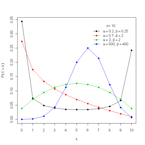
    This distribution is called the beta-binomial distribution. Below is an image from Wikipedia showing a graph of \(p(X)\) for \(N=10\) and a number of different values of \(a\) and \(b\). You can see that, especially for small value of \(a\) and \(b\) the distribution is a lot more spread out than the binomial distribution. This is because there is randomness coming from both \(\rho\) and the binomial conditional distribution.

    A plot of the beta-binomial distribution for different values of the parameters a and b. For small values of a and b, the distribution is very spread out.
  • Two sample tests as correlation tests

    Suppose we have two samples \(Y_1^{(0)}, Y_2^{(0)},\ldots, Y_{n_0}^{(0)}\) and \(Y_1^{(1)},Y_2^{(1)},\ldots, Y_{n_1}^{(1)}\) and we want to test if they are from the same distribution. Many popular tests can be reinterpreted as correlation tests by pooling the two samples and introducing a dummy variable that encodes which sample each data point comes from. In this post we will see how this plays out in a simple t-test.

    The equal variance t-test

    In the equal variance t-test, we assume that \(Y_i^{(0)} \stackrel{\text{iid}}{\sim} \mathcal{N}(\mu_0,\sigma^2)\) and \(Y_i^{(1)} \stackrel{\text{iid}}{\sim} \mathcal{N}(\mu_1,\sigma^2)\), where \(\sigma^2\) is unknown. Our hypothesis that \(Y_1^{(0)}, Y_2^{(0)},\ldots, Y_{n_0}^{(0)}\) and \(Y_1^{(1)},Y_2^{(1)},\ldots, Y_{n_1}^{(1)}\) are from the same distribution becomes the hypothesis \(\mu_0 = \mu_1\). The test statistic is

    \(t = \frac{\displaystyle \overline{Y}^{(1)} – \overline{Y}^{(0)}}{\displaystyle \hat{\sigma}\sqrt{\frac{1}{n_0}+\frac{1}{n_1}}}\),

    where \(\overline{Y}^{(0)}\) and \(\overline{Y}^{(1)}\) are the two sample means. The variable \(\hat{\sigma}\) is the pooled estimate of the standard deviation and is given by

    \(\hat{\sigma}^2 = \displaystyle\frac{1}{n_0+n_1-2}\left(\sum_{i=1}^{n_0}\left(Y_i^{(0)}-\overline{Y}^{(0)}\right)^2 + \sum_{i=1}^{n_1}\left(Y_i^{(1)}-\overline{Y}^{(1)}\right)^2\right)\).

    Under the null hypothesis, \(t\) follows the T-distribution with \(n_0+n_1-2\) degrees of freedom. We thus reject the null \(\mu_0=\mu_1\) when \(|t|\) exceeds the \(1-\alpha/2\) quantile of the T-distribution.

    Pooling the data

    We can turn this two sample test into a correlation test by pooling the data and using a linear model. Let \(Y_1,\ldots,Y_{n_0}, Y_{n_0+1},\ldots,Y_{n_0+n_1}\) be the pooled data and for \(i = 1,\ldots, n_0+n_1\), define \(x_i \in \{0,1\}\) by

    \(x_i = \begin{cases} 0 & \text{if } 1 \le i \le n_0,\\ 1 & \text{if } n_0+1 \le i \le n_0+n_1.\end{cases}\)

    The assumptions that \(Y_i^{(0)} \stackrel{\text{iid}}{\sim} \mathcal{N}(\mu_0,\sigma^2)\) and \(Y_i^{(1)} \stackrel{\text{iid}}{\sim} \mathcal{N}(\mu_1,\sigma^2)\) can be rewritten as

    \(Y_i = \beta_0+\beta_1x_i + \varepsilon_i,\)

    where \(\varepsilon_i \stackrel{\text{iid}}{\sim} \mathcal{N}(0,\sigma^2)\). That is, we have expressed our modelling assumptions as a linear model. When working with this linear model, the hypothesis \(\mu_0 = \mu_1\) is equivalent to \(\beta_1 = 0\). To test \(\beta_1 = 0\) we can use the standard t-test for a coefficient in linear model. The test statistic in this case is

    \(t’ = \displaystyle\frac{\hat{\beta}_1}{\hat{\sigma}_{OLS}\sqrt{(X^TX)^{-1}_{11}}},\)

    where \(\hat{\beta}_1\) is the ordinary least squares estimate of \(\beta_1\), \(X \in \mathbb{R}^{(n_0+n_1)\times 2}\) is the design matrix and \(\hat{\sigma}_{OLS}\) is an estimate of \(\sigma\) given by

    \(\hat{\sigma}_{OLS}^2 = \displaystyle\frac{1}{n_0+n_1-2}\sum_{i=1}^{n_0+n_1} (Y_i-\hat{Y}_i)^2,\)

    where \(\hat{Y} = \hat{\beta}_0+\hat{\beta}_1x_i\) is the fitted value of \(Y_i\).

    It turns out that \(t’\) is exactly equal to \(t\). We can see this by writing out the design matrix and calculating everything above. The design matrix has rows \([1,x_i]\) and is thus equal to

    \(X = \begin{bmatrix} 1&x_1\\ 1&x_2\\ \vdots&\vdots\\ 1&x_{n_0}\\ 1&x_{n_0+1}\\ \vdots&\vdots\\ 1&x_{n_0+n_1}\end{bmatrix} = \begin{bmatrix} 1&0\\ 1&0\\ \vdots&\vdots\\ 1&0\\ 1&1\\ \vdots&\vdots\\ 1&1\end{bmatrix}.\)

    This implies that

    \(X^TX = \begin{bmatrix} n_0+n_1 &n_1\\n_1&n_1 \end{bmatrix},\)

    And therefore,

    \((X^TX)^{-1} = \frac{1}{(n_0+n_1)n_1-n_1^2}\begin{bmatrix} n_1 &-n_1\\-n_1&n_0+n_1 \end{bmatrix} = \frac{1}{n_0n_1}\begin{bmatrix} n_1&-n_1\\-n_1&n_0+n_1\end{bmatrix} =\begin{bmatrix} \frac{1}{n_0}&-\frac{1}{n_0}\\-\frac{1}{n_0}&\frac{1}{n_0}+\frac{1}{n_1}\end{bmatrix} .\)

    Thus, \((X^TX)^{-1}_{11} = \frac{1}{n_0}+\frac{1}{n_1}\). So,

    \(t’ = \displaystyle\frac{\hat{\beta}_1}{\hat{\sigma}_{OLS}\sqrt{\frac{1}{n_0}+\frac{1}{n_1}}},\)

    which is starting to like \(t\) from the two-sample test. Now

    \(X^TY = \begin{bmatrix} \displaystyle\sum_{i=1}^{n_0+n_1} Y_i\\ \displaystyle \sum_{i=n_0+1}^{n_0+n_1} Y_i \end{bmatrix} = \begin{bmatrix} n_0\overline{Y}^{(0)} + n_1\overline{Y}^{(1)}\\ n_1\overline{Y}^{(1)} \end{bmatrix}.\)

    And so

    \(\hat{\beta} = (X^TX)^{-1}X^TY = \begin{bmatrix} \frac{1}{n_0}&-\frac{1}{n_0}\\-\frac{1}{n_0}&\frac{1}{n_0}+\frac{1}{n_1}\end{bmatrix}\begin{bmatrix} n_0\overline{Y}^{(0)} + n_1\overline{Y}^{(1)}\\ n_1\overline{Y}^{(1)} \end{bmatrix}=\begin{bmatrix} \overline{Y}^{(0)}\\ \overline{Y}^{(1)} -\overline{Y}^{(0)}\end{bmatrix}.\)

    Thus, \(\hat{\beta}_1 = \overline{Y}^{(1)} -\overline{Y}^{(0)}\) and

    \(t’ = \displaystyle\frac{\overline{Y}^{(1)}-\overline{Y}^{(0)}}{\hat{\sigma}_{OLS}\sqrt{\frac{1}{n_0}+\frac{1}{n_1}}}.\)

    This means to show that \(t’ = t\), we only need to show that \(\hat{\sigma}_{OLS}^2=\hat{\sigma}^2\). To do this, note that the fitted values \(\hat{Y}\) are equal to

    \(\displaystyle\hat{Y}_i=\hat{\beta}_0+x_i\hat{\beta}_1 = \begin{cases} \overline{Y}^{(0)} & \text{if } 1 \le i \le n_0,\\ \overline{Y}^{(1)} & \text{if } n_0+1\le i \le n_0+n_1\end{cases}.\)

    Thus,

    \(\hat{\sigma}^2_{OLS} = \displaystyle\frac{1}{n_0+n_1-2}\sum_{i=1}^{n_0+n_1}\left(Y_i-\hat{Y}_i\right)^2=\displaystyle\frac{1}{n_0+n_1-2}\left(\sum_{i=1}^{n_0}\left(Y_i^{(0)}-\overline{Y}^{(0)}\right)^2 + \sum_{i=1}^{n_1}\left(Y_i^{(1)}-\overline{Y}^{(1)}\right)^2\right),\)

    Which is exactly \(\hat{\sigma}^2\). Therefore, \(t’=t\) and the two sample t-test is equivalent to a correlation test.

    The Friedman-Rafsky test

    In the above example, we saw that the two sample t-test was a special case of the t-test for regressions. This is neat but both tests make very strong assumptions about the data. However, the same thing happens in a more interesting non-parametric setting.

    In their 1979 paper, Jerome Friedman and Lawrence Rafsky introduced a two sample tests that makes no assumptions about the distribution of the data. The two samples do not even have to real-valued and can instead be from any metric space. It turns out that their test is a special case of another procedure they devised for testing for association (Friedman & Rafsky, 1983). As with the t-tests above, this connection comes from pooling the two samples and introducing a dummy variable.

    I plan to write a follow up post explaining these procedures but you can also read about it in Chapter 6 of Group Representations in Probability and Statistics by Persi Diaconis.

    References

    Persi Diaconis “Group representations in probability and statistics,” pp 104-106, Hayward, CA: Institute of Mathematical Statistics, (1988)

    Jerome H. Friedman, Lawrence C. Rafsky “Multivariate Generalizations of the Wald-Wolfowitz and Smirnov Two-Sample Tests,” The Annals of Statistics, Ann. Statist. 7(4), 697-717, (July, 1979)

    Jerome H. Friedman, Lawrence C. Rafsky “Graph-Theoretic Measures of Multivariate Association and Prediction,” The Annals of Statistics, Ann. Statist. 11(2), 377-391, (June, 1983).

  • MCMC for hypothesis testing

    A Monte Carlo significance test of the null hypothesis \(X_0 \sim H\) requires creating independent samples \(X_1,\ldots,X_B \sim H\). The idea is if \(X_0 \sim H\) and independently \(X_1,\ldots,X_B\) are i.i.d. from \(H\), then for any test statistic \(T\), the rank of \(T(X_0)\) among \(T(X_0), T(X_1),\ldots, T(X_B)\) is uniformly distributed on \(\{1,\ldots, B+1\}\). This means that if \(T(X_0)\) is one of the \(k\) largest values of \(T(X_b)\), then we can reject the hypothesis \(X \sim H\) at the significance level \(k/(B+1)\).

    The advantage of Monte Carlo significance tests is that we do not need an analytic expression for the distribution of \(T(X_0)\) under \(X_0 \sim H\). By generating the i.i.d. samples \(X_1,\ldots,X_B\), we are making an empirical distribution that approximates the theoretical distribution. However, sometimes sampling \(X_1,\ldots, X_B\) is just as intractable as theoretically studying the distribution of \(T(X_0)\) . Often approximate samples based on Markov chain Monte Carlo (MCMC) are used instead. However, these samples are not independent and may not be sampling from the true distribution. This means that a test using MCMC may not be statistically valid

    In the 1989 paper Generalized Monte Carlo significance tests, Besag and Clifford propose two methods that solve this exact problem. Their two methods can be used in the same settings where MCMC is used but they are statistically valid and correctly control the Type 1 error. In this post, I will describe just one of the methods – the serial test.

    Background on Markov chains

    To describe the serial test we will need to introduce some notation. Let \(P\) denote a transition matrix for a Markov chain on a discrete state space \(\mathcal{X}.\) A Markov chain with transition matrix \(P\) thus satisfies,

    \(\mathbb{P}(X_n = x_n \mid X_0 = x_0,\ldots, X_{n-1} = x_{n-1}) = P(x_{n-1}, x_n)\)

    Suppose that the transition matrix \(P\) has a stationary distribution \(\pi\). This means that if \((X_0, X_1,\ldots)\) is a Markov chain with transition matrix \(P\) and \(X_0\) is distributed according to \(\pi\), then \(X_1\) is also distributed according to \(\pi\). This implies that all \(X_i\) are distributed according to \(\pi\).

    We can construct a new transition matrix \(Q\) from \(P\) and \(\pi\) by \(Q(y,x) = P(x,y) \frac{\pi(x)}{\pi(y)}\). The transition matrix \(Q\) is called the reversal of \(P\). This is because for all \(x\) and \(y\) in \(\mathcal{X}\), \(\pi(x)P(x,y) = \pi(y)Q(x,y)\). That is the chance of drawing \(x\) from \(\pi\) and then transitioning to \(y\) according to \(P\) is equal to the chance of drawing \(y\) from \(\pi\) and then transitioning to \(x\) according to \(Q\)

    The new transition matrix \(Q\) also allows us to reverse longer runs of the Markov chain. Fix \(n \ge 0\) and let \((X_0,X_1,\ldots,X_n)\) be a Markov chain with transition matrix \(P\) and initial distribution \(\pi\). Also let \((Y_0,Y_1,\ldots,Y_n)\) be a Markov chain with transition matrix \(Q\) and initial distribution \(\pi\), then

    \((X_0,X_1,\ldots,X_{n-1}, X_n) \stackrel{dist}{=} (Y_n,Y_{n-1},\ldots, Y_1,Y_0) \),

    where \(\stackrel{dist}{=}\) means equal in distribution.

    The serial test

    Suppose we want to test the hypothesis \(x \sim \pi\) where \(x \in \mathcal{X}\) is our observed data and \(\pi\) is some distribution on \(\mathcal{X}\). To conduct the serial test, we need to construct a Markov chain \(P\) for which \(\pi\) is a stationary distribution. We then also need to construct the reversal \(Q\) described above. There are many possible ways to construct \(P\) such as the Metropolis-Hastings algorithm.

    We also need a test statistic \(T\). This is a function \(T:\mathcal{X} \to \mathbb{R}\) which we will use to detect outliers. This function is the same function we would use in a regular Monte Carlo test. Namely, we want to reject the null hypothesis when \(T(x)\) is much larger than we would expect under \(x \sim \pi\).

    The serial test then proceeds as follows. First we pick \(\xi\) uniformly in \(\{0,1,\ldots,B\}\) and set \(X_\xi = x\). We then generate \((X_\xi, X_{\xi+1},\ldots,X_B)\) as a Markov chain with transition matrix \(P\) that starts at \(X_\xi = x\). Likewise we generate \((X_\xi, X_{\xi-1},\ldots, X_0)\) as a Markov chain that starts from \(Q\).

    We then apply \(T\) to each of \((X_0,X_1,\ldots,X_\xi,\ldots,X_B)\) and count the number of \(b \in \{0,1,\ldots,B\}\) such that \(T(X_b) \ge T(X_\xi) = T(x)\). If there are \(k\) such \(b\), then the reported p-value of our test is \(k/(B+1)\).

    We will now show that this test produces a valid p-value. That is, when \(x \sim \pi\), the probability that \(k/(B+1)\) is less than \(\alpha\) is at most \(\alpha\). In symbols,

    \(\mathbb{P}\left( \frac{\#\{b: T(X_b) \ge T(X_\xi)\}}{B+1} \le \alpha \right) \le \alpha\)

    Under the null hypothesis \(x \sim \pi\), \((X_\xi, X_{\xi-1},\ldots, X_0)\) is equal in distribution to generating \(X_0\) from \(\pi\) and using the transition matrix \(P\) to go from \(X_i\) to \(X_{i+1}\).

    Thus, under the null hypothesis, the distribution of \((X_0,X_1,\ldots,X_B)\) does not depend on \(\xi\). The entire procedure is equivalent to generating a Markov chain \(\mathbf{X} = (X_0,X_1,\ldots,X_B)\) with initial distribution \(\pi\) and transition matrix \(P\), and then choosing \(\xi \in \{0,1,\ldots,B\}\) independently of \(\mathbf{X}\). This is enough to show that the serial method produces valid p-values. The idea is that since the distribution of \(\mathbf{X}\) does not depend on \(\xi\) and \(\xi\) is uniformly distributed on \(\{0,1,\ldots,B\}\), the probability that \(T(X_\xi)\) is in the top \(\alpha\) proportion of \(T(X_b)\) should be at most \(\alpha\). This is proved more formally below.

    For each \(i \in \{0,1,\ldots,B\}\), let \(A_i\) be the event that \(T(X_i)\) is in the top \(\alpha\) proportion of \(T(X_0),\ldots,T(X_B)\). That is,

    \(A_i = \left\{ \frac{\# \{b : T(X_b) \ge T(X_i)\} }{B+1} \le \alpha \right\}\).

    Let \(I_{A_i}\) be the indicator function for the event \(A_i\). Since at must \(\alpha(B+1)\) values of \(i\) can be in the top \(\alpha\) fraction of \(T(X_0),\ldots,T(X_B)\), we have that

    \(\sum_{i=0}^B I_{A_i} \le \alpha(B+1)\),

    Therefor, by linearity of expectations,

    \(\sum_{i=0}^B \mathbb{P}(A_i) \le \alpha(B+1)\)

    By the law of total probability we have,

    \(\mathbb{P}\left(\frac{\#\{b: T(X_b) \ge T(X_\xi)\}}{B+1} \le \alpha \right) = \sum_{i=0}^B \mathbb{P}\left(\frac{\#\{b: T(X_b) \ge T(X_\xi)\}}{B+1} \le \alpha | \xi = i\right)\mathbb{P}(\xi = i)\),

    Since \(\xi\) is uniform on \(\{0,\ldots,B\}\), \(\mathbb{P}(\xi = i)\) is \(\frac{1}{B+1}\) for all \(i\). Furthermore, by independence of \(\xi\) and \(\mathbf{X}\), we have

    \(\mathbb{P}\left(\frac{\#\{b: T(X_b) \ge T(X_\xi)\}}{B+1} \le \alpha | \xi = i\right) = \mathbb{P}\left(\frac{\#\{b: T(X_b) \ge T(X_i)\}}{B+1} \le \alpha | \xi = i\right) = \mathbb{P}(A_i)\).

    Thus, by our previous bound,

    \(\mathbb{P}\left(\frac{\#\{b: T(X_b) \ge T(X_\xi)\}}{B+1} \le \alpha \right) = \frac{1}{B+1}\sum_{i=0}^B \mathbb{P}(A_i) \le \alpha\).

    Applications

    In the original paper by Besag and Clifford, the authors discuss how this procedure can be used to perform goodness-of-fit tests. They construct Markov chains that can test the Rasch model or the Ising model. More broadly the method can be used to tests goodness-of-fit tests for any exponential family by using the Markov chains developed by Diaconis and Sturmfels.

    A similar method has also been applied more recently to detect Gerrymandering. In this setting, the null hypothesis is the uniform distribution on all valid redistrictings of a state and the test statistics \(T\) measure the political advantage of a given districting.

    References

    1. Besag, Julian, and Peter Clifford. “Generalized Monte Carlo Significance Tests.” Biometrika 76, no. 4 (1989)
    2. Persi Diaconis, Bernd Sturmfels “Algebraic algorithms for sampling from conditional distributions,” The Annals of Statistics, Ann. Statist. 26(1), 363-397, (1998)
    3. Chikina, Maria et al. “Assessing significance in a Markov chain without mixing.” Proceedings of the National Academy of Sciences of the United States of America vol. 114,11 (2017)
  • Sampling from the non-central chi-squared distribution

    The non-central chi-squared distribution is a generalisation of the regular chi-squared distribution. The chi-squared distribution turns up in many statistical tests as the (approximate) distribution of a test statistic under the null hypothesis. Under alternative hypotheses, those same statistics often have approximate non-central chi-squared distributions.

    This means that the non-central chi-squared distribution is often used to study the power of said statistical tests. In this post I give the definition of the non-central chi-squared distribution, discuss an important invariance property and show how to efficiently sample from this distribution.

    Definition

    Let \(Z\) be a normally distributed random vector with mean \(0\) and covariance \(I_n\). Given a vector \(\mu \in \mathbb{R}^n\), the non-central chi-squared distribution with \(n\) degrees of freedom and non-centrality parameter \(\Vert \mu\Vert_2^2\) is the distribution of the quantity

    \(\Vert Z+\mu \Vert_2^2 = \sum\limits_{i=1}^n (Z_i+\mu_i)^2. \)

    This distribution is denoted by \(\chi^2_n(\Vert \mu \Vert_2^2)\). As this notation suggests, the distribution of \(\Vert Z+\mu \Vert_2^2\) depends only on \(\Vert \mu \Vert_2^2\), the norm of \(\mu\). The first few times I heard this fact, I had no idea why it would be true (and even found it a little spooky). But, as we will see below, the result is actually a simply consequence of the fact that standard normal vectors are invariant under rotations.

    Rotational invariance

    Suppose that we have two vectors \(\mu, \nu \in \mathbb{R}^n\) such that \(\Vert \mu\Vert_2^2 = \Vert \nu \Vert_2^2\). We wish to show that if \(Z \sim \mathcal{N}(0,I_n)\), then

    \(\Vert Z+\mu \Vert_2^2\) has the same distribution as \(\Vert Z + \nu \Vert_2^2\).

    Since \(\mu\) and \(\nu\) have the same norm there exists an orthogonal matrix \(U \in \mathbb{R}^{n \times n}\) such that \(U\mu = \nu\). Since \(U\) is orthogonal and \(Z \sim \mathcal{N}(0,I_n)\), we have \(Z’=UZ \sim \mathcal{N}(U0,UU^T) = \mathcal{N}(0,I_n)\). Furthermore, since \(U\) is orthogonal, \(U\) preserves the norm \(\Vert \cdot \Vert_2^2\). This is because, for all \(x \in \mathbb{R}^n\),

    \(\Vert Ux\Vert_2^2 = (Ux)^TUx = x^TU^TUx=x^Tx=\Vert x\Vert_2^2.\)

    Putting all these pieces together we have

    \(\Vert Z+\mu \Vert_2^2 = \Vert U(Z+\mu)\Vert_2^2 = \Vert UZ + U\mu \Vert_2^2 = \Vert Z’+\nu \Vert_2^2\).

    Since \(Z\) and \(Z’\) have the same distribution, we can conclude that \( \Vert Z’+\nu \Vert_2^2\) has the same distribution as \(\Vert Z + \nu \Vert\). Since \(\Vert Z + \mu \Vert_2^2 = \Vert Z’+\nu \Vert_2^2\), we are done.

    Sampling

    Above we showed that the distribution of the non-central chi-squared distribution, \(\chi^2_n(\Vert \mu\Vert_2^2)\) depends only on the norm of the vector \(\mu\). We will now use this to provide an algorithm that can efficiently generate samples from \(\chi^2_n(\Vert \mu \Vert_2^2)\).

    A naive way to sample from \(\chi^2_n(\Vert \mu \Vert_2^2)\) would be to sample \(n\) independent standard normal random variables \(Z_i\) and then return \(\sum_{i=1}^n (Z_i+\mu_i)^2\). But for large values of \(n\) this would be very slow as we have to simulate \(n\) auxiliary random variables \(Z_i\) for each sample from \(\chi^2_n(\Vert \mu \Vert_2^2)\). This approach would not scale well if we needed many samples.

    An alternative approach uses the rotation invariance described above. The distribution \(\chi^2_n(\Vert \mu \Vert_2^2)\) depends only on \(\Vert \mu \Vert_2^2\) and not directly on \(\mu\). Thus, given \(\mu\), we could instead work with \(\nu = \Vert \mu \Vert_2 e_1\) where \(e_1\) is the vector with a \(1\) in the first coordinate and \(0\)s in all other coordinates. If we use \(\nu\) instead of \(\mu\), we have

    \(\sum\limits_{i=1}^n (Z_i+\nu_i)^2 = (Z_1+\Vert \mu \Vert_2)^2 + \sum\limits_{i=2}^{n}Z_i^2.\)

    The sum \(\sum_{i=2}^n Z_i^2\) follows the regular chi-squared distribution with \(n-1\) degrees of freedom and is independent of \(Z_1\). The regular chi-squared distribution is a special case of the gamma distribution and can be effectively sampled with rejection sampling for large shape parameter (see here).

    The shape parameter for \(\sum_{i=2}^n Z_i^2\) is \(\frac{n-1}{2}\), so for large values of \(n\) we can efficiently sample a value \(Y\) that follows that same distribution as \(\sum_{i=2}^n Z_i^2 \sim \chi^2_{n-1}\). Finally to get a sample from \(\chi^2_n(\Vert \mu \Vert_2^2)\) we independently sample \(Z_1\), and then return the sum \((Z_1+\Vert \mu\Vert_2)^2 +Y\).

    Conclusion

    In this post, we saw that the rotational invariance of the standard normal distribution gives a similar invariance for the non-central chi-squared distribution.

    This invariance allowed us to efficiently sample from the non-central chi-squared distribution. The sampling procedure worked by reducing the problem to sampling from the regular chi-squared distribution.

    The same invariance property is also used to calculate the cumulative distribution function and density of the non-central chi-squared distribution. Although the resulting formulas are not for the faint of heart.

  • The Singular Value Decomposition (SVD)

    The singular value decomposition (SVD) is a powerful matrix decomposition. It is used all the time in statistics and numerical linear algebra. The SVD is at the heart of the principal component analysis, it demonstrates what’s going on in ridge regression and it is one way to construct the Moore-Penrose inverse of a matrix. For more SVD love, see the tweets below.

    A tweet by Women in Statistics and Data Science about the SVD.
    The full thread is here https://twitter.com/WomenInStat/status/1285610321747611653?s=20&t=Elj62mGSc9gINHvbwt82Zw

    In this post I’ll define the SVD and prove that it always exists. At the end we’ll look at some pictures to better understand what’s going on.

    Definition

    Let \(X\) be a \(n \times p\) matrix. We will define the singular value decomposition first in the case \(n \ge p\). The SVD consists of three matrix \(U \in \mathbb{R}^{n \times p}, \Sigma \in \mathbb{R}^{p \times p}\) and \(V \in \mathbb{R}^{p \times p}\) such that \(X = U\Sigma V^T\). The matrix \(\Sigma\) is required to be diagonal with non-negative diagonal entries \(\sigma_1 \ge \sigma_2 \ge \ldots \ge \sigma_p \ge 0\). These numbers are called the singular values of \(X\). The matrices \(U\) and \(V\) are required to orthogonal matrices so that \(U^TU=V^TV = I_p\), the \(p \times p\) identity matrix. Note that since \(V\) is square we also have \(VV^T=I_p\) however we won’t have \(UU^T = I_n\) unless \(n = p\).

    In the case when \(n \le p\), we can define the SVD of \(X\) in terms of the SVD of \(X^T\). Let \(\widetilde{U} \in \mathbb{R}^{p \times n}, \widetilde{\Sigma} \in \mathbb{R}^{n \times n}\) and \(\widetilde{V} \in \mathbb{R}^{n \times n}\) be the SVD of \(X^T\) so that \(X^T=\widetilde{U}\widetilde{\Sigma}\widetilde{V}^T\). The SVD of \(X\) is then given by transposing both sides of this equation giving \(U = \widetilde{V}, \Sigma = \widetilde{\Sigma}^T=\widetilde{\Sigma}\) and \(V = \widetilde{U}\).

    Construction

    The SVD of a matrix can be found by iteratively solving an optimisation problem. We will first describe an iterative procedure that produces matrices \(U \in \mathbb{R}^{n \times p}, \Sigma \in \mathbb{R}^{p \times p}\) and \(V \in \mathbb{R}^{p \times p}\). We will then verify that \(U,\Sigma \) and \(V\) satisfy the defining properties of the SVD.

    We will construct the matrices \(U\) and \(V\) one column at a time and we will construct the diagonal matrix \(\Sigma\) one entry at a time. To construct the first columns and entries, recall that the matrix \(X\) is really a linear function from \(\mathbb{R}^p\) to \(\mathbb{R}^n\) given by \(v \mapsto Xv\). We can thus define the operator norm of \(X\) via

    \(\Vert X \Vert = \sup\left\{ \|Xv\|_2 : \|v\|_2 =1\right\},\)

    where \(\|v\|_2\) represents the Euclidean norm of \(v \in \mathbb{R}^p\) and \(\|Xv\|_2\) is the Euclidean norm of \(Xv \in \mathbb{R}^n\). The set of vectors \(\{v \in \mathbb{R} : \|v\|_2 = 1 \}\) is a compact set and the function \(v \mapsto \|Xv\|_2\) is continuous. Thus, the supremum used to define \(\Vert X \Vert\) is achieved at some vector \(v_1 \in \mathbb{R}^p\). Define \(\sigma_1 = \|X v_1\|_2\). If \(\sigma_1 \neq 0\), then define \(u_1 = Xv_1/\sigma_1 \in \mathbb{R}^n\). If \(\sigma_1 = 0\), then define \(u_1\) to be an arbitrary vector in \(\mathbb{R}^n\) with \(\|u\|_2 = 1\). To summarise we have

    • \(v_1 \in \mathbb{R}^p\) with \(\|v_1\|_2 = 1\).
    • \(\sigma_1 = \|X\| = \|Xv_1\|_2\).
    • \(u_1 \in \mathbb{R}^n\) with \(\|u_1\|_2=1\) and \(Xv_1 = \sigma_1u_1\).

    We have now started to fill in our SVD. The number \(\sigma_1 \ge 0\) is the first singular value of \(X\) and the vectors \(v_1\) and \(u_1\) will be the first columns of the matrices \(V\) and \(U\) respectively.

    Now suppose that we have found the first \(k\) singular values \(\sigma_1,\ldots,\sigma_k\) and the first \(k\) columns of \(V\) and \(U\). If \(k = p\), then we are done. Otherwise we repeat a similar process.

    Let \(v_1,\ldots,v_k\) and \(u_1,\ldots,u_k\) be the first \(k\) columns of \(V\) and \(U\). The vectors \(v_1,\ldots,v_k\) split \(\mathbb{R}^p\) into two subspaces. These subspaces are \(S_1 = \text{span}\{v_1,\ldots,v_k\}\) and \(S_2 = S_1^\perp\), the orthogonal compliment of \(S_1\). By restricting \(X\) to \(S_2\) we get a new linear map \(X_{|S_2} : S_2 \to \mathbb{R}^n\). Like before, the operator norm of \(X_{|S_2}\) is defined to be

    \(\|X_{|S_2}\| = \sup\{\|X_{|S_2}v\|_2:v \in S_2, \|v\|_2=1\}\).

    Since \(S_2 = \text{span}\{v_1,\ldots,v_k\}^\perp\) we must have

    \(\|X_{|S_2}\| = \sup\{\|Xv\|_2:v \in \mathbb{R}^p, \|v\|_2=1, v_j^Tv = 0 \text{ for } j=1,\ldots,k\}.\)

    The set \(\{v \in \mathbb{R}^p : \|v\|_2=1, v_j^Tv=0\text{ for } j=1,\ldots,k\}\) is a compact set and thus there exists a vector \(v_{k+1}\) such that \(\|Xv_{k+1}\|_2 = \|X_{|S_2}\|\). As before define \(\sigma_{k+1} = \|Xv_{k+1}\|_2\) and \(u_{k+1} = Xv_{k+1}/\sigma_{k+1}\) if \(\sigma_{k+1}\neq 0\). If \(\sigma_{k+1} = 0\), then define \(u_{k+1}\) to be any vector in \(\mathbb{R}^{n}\) that is orthogonal to \(u_1,u_2,\ldots,u_k\).

    This process repeats until eventually \(k = p\) and we have produced matrices \(U \in \mathbb{R}^{n \times p}, \Sigma \in \mathbb{R}^{p \times p}\) and \(V \in \mathbb{R}^{p \times p}\). In the next section, we will argue that these three matrices satisfy the properties of the SVD.

    Correctness

    The defining properties of the SVD were given at the start of this post. We will see that most of the properties follow immediately from the construction but one of them requires a bit more analysis. Let \(U = [u_1,\ldots,u_p]\), \(\Sigma = \text{diag}(\sigma_1,\ldots,\sigma_p)\) and \(V= [v_1,\ldots,v_p]\) be the output from the above construction.

    First note that by construction \(v_1,\ldots, v_p\) are orthogonal since we always had \(v_{k+1} \in \text{span}\{v_1,\ldots,v_k\}^\perp\). It follows that the matrix \(V\) is orthogonal and so \(V^TV=VV^T=I_p\).

    The matrix \(\Sigma\) is diagonal by construction. Furthermore, we have that \(\sigma_{k+1} \le \sigma_k\) for every \(k\). This is because both \(\sigma_k\) and \(\sigma_{k+1}\) were defined as maximum value of \(\|Xv\|_2\) over different subsets of \(\mathbb{R}^p\). The subset for \(\sigma_k\) contained the subset for \(\sigma_{k+1}\) and thus \(\sigma_k \ge \sigma_{k+1}\).

    We’ll next verify that \(X = U\Sigma V^T\). Since \(V\) is orthogonal, the vectors \(v_1,\ldots,v_p\) form an orthonormal basis for \(\mathbb{R}^p\). It thus suffices to check that \(Xv_k = U\Sigma V^Tv_k\) for \(k = 1,\ldots,p\). Again by the orthogonality of \(V\) we have that \(V^Tv_k = e_k\), the \(k^{th}\) standard basis vector. Thus,

    \(U\Sigma V^Tv_k = U\Sigma e_k = U\sigma_k e_k = \sigma_k u_k.\)

    Above, we used that \(\Sigma\) was a diagonal matrix and that \(u_k\) is the \(k^{th}\) column of \(U\). If \(\sigma_k \neq 0\), then \(\sigma_k u_k = Xv_k\) by definition. If \(\sigma_k =0\), then \(\|Xv_k\|_2=0\) and so \(Xv_k = 0 = \sigma_ku_k\) also. Thus, in either case, \(U\Sigma V^Tv_k = Xv_k\) and so \(U\Sigma V^T = X\).

    The last property we need to verify is that \(U\) is orthogonal. Note that this isn’t obvious. At each stage of the process, we made sure that \(v_{k+1} \in \text{span}\{v_1,\ldots,v_k\}^\perp\). However, in the case that \(\sigma_{k+1} \neq 0\), we simply defined \(u_{k+1} = Xv_{k+1}/\sigma_{k+1}\). It is not clear why this would imply that \(u_{k+1}\) is orthogonal to \(u_1,\ldots,u_k\).

    It turns out that a geometric argument is needed to show this. The idea is that if \(u_{k+1}\) was not orthogonal to \(u_j\) for some \(j \le k\), then \(v_j\) couldn’t have been the value that maximises \(\|Xv\|_2\).

    Let \(u_{k}\) and \(u_j\) be two columns of \(U\) with \(j < k\) and \(\sigma_j,\sigma_k > 0\). We wish to show that \(u_j^Tu_k = 0\). To show this we will use the fact that \(v_j\) and \(v_k\) are orthonormal and perform “polar-interpolation“. That is, for \(\lambda \in [0,1]\), define

    \(v_\lambda = \sqrt{1-\lambda}\cdot v_{j}-\sqrt{\lambda} \cdot v_k.\)

    Since \(v_{j}\) and \(v_k\) are orthogonal, we have that

    \(\|v_\lambda\|_2^2 = (1-\lambda)\|v_{j}\|_2^2+\lambda\|v_k\|_2^2 = (1-\lambda)+\lambda = 1.\)

    Furthermore \(v_\lambda\) is orthogonal to \(v_1,\ldots,v_{j-1}\). Thus, by definition of \(v_j\),

    \(\|Xv_\lambda\|_2^2 \le \sigma_j^2 = \|Xv_j\|_2^2.\)

    By the linearity of \(X\) and the definitions of \(u_j,u_k\),

    \(\|Xv_\lambda\|_2^2 = \|\sqrt{1-\lambda}\cdot Xv_j+\sqrt{\lambda}\cdot Xv_{k+1}\|_2^2 = \|\sigma_j\sqrt{1-\lambda}\cdot u_j+\sigma_{k+1}\sqrt{\lambda}\cdot u_{k+1}\|_2^2\).

    Since \(Xv_j = \sigma_ju_j\) and \(Xv_{k+1}=\sigma_{k+1}u_{k+1}\), we have

    \((1-\lambda)\sigma_j^2 + 2\sqrt{\lambda(1-\lambda)}\cdot \sigma_1\sigma_2 u_j^Tu_{k}+\lambda\sigma_k^2 = \|Xv_\lambda\|_2^2 \le \sigma_j^2\)

    Rearranging and dividing by \(\sqrt{\lambda}\) gives,

    \(2\sqrt{1-\lambda}\cdot \sigma_1\sigma_2 u_j^Tu_k \le \sqrt{\lambda}\cdot(\sigma_j^2-\sigma_k^2).\) for all \(\lambda \in (0,1]\)

    Taking \(\lambda \searrow 0\) gives \(u_j^Tu_k \le 0\). Performing the same polar interpolation with \(v_\lambda’ = \sqrt{1-\lambda}v_j – \sqrt{\lambda}v_k\) shows that \(-u_j^Tu_k \le 0\) and hence \(u_j^Tu_k = 0\).

    We have thus proved that \(U\) is orthogonal. This proof is pretty “slick” but it isn’t very illuminating. To better demonstrate the concept, I made an interactive Desmos graph that you can access here.

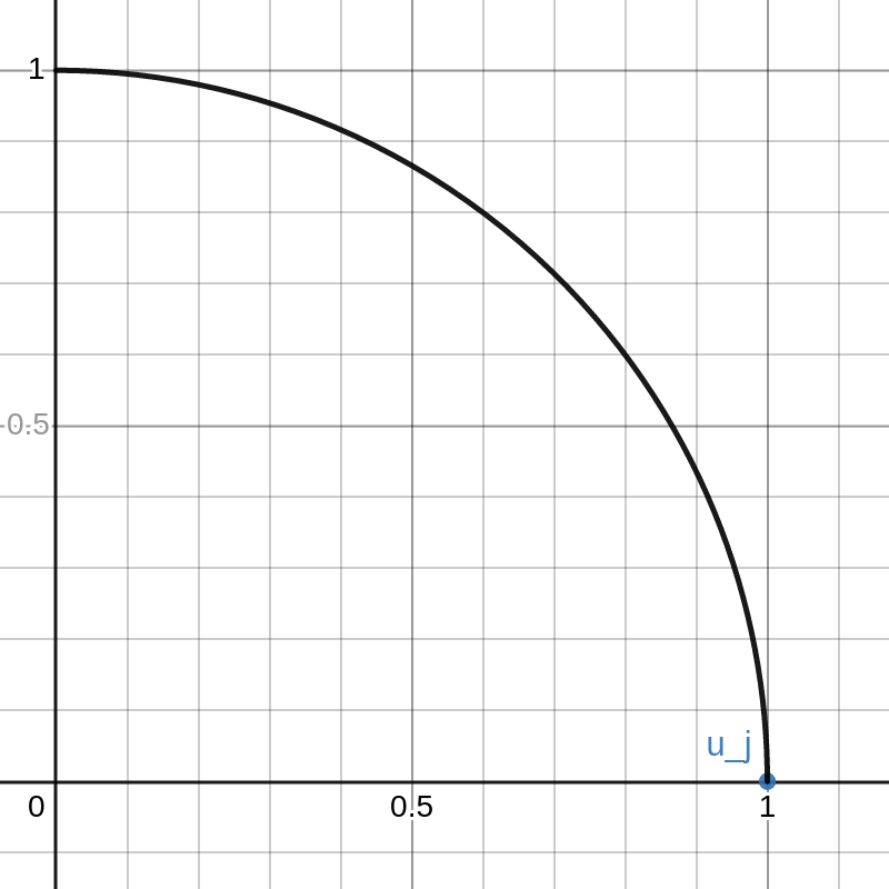
    This graph shows example vectors \(u_j, u_k \in \mathbb{R}^2\). The vector \(u_j\) is fixed at \((1,0)\) and a quarter circle of radius \(1\) is drawn. Any vectors \(u\) that are outside this circle have \(\|u\|_2 > 1 = \|u_j\|_2\).

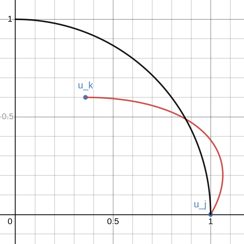
    The vector \(u_k\) can be moved around inside this quarter circle. This can be done either cby licking and dragging on the point or changing that values of \(a\) and \(b\) on the left. The red curve is the path of

    \(\lambda \mapsto \sqrt{1-\lambda}\cdot u_j+\sqrt{\lambda}\cdot u_k\).

    As \(\lambda\) goes from \(0\) to \(1\), the path travels from \(u_j\) to \(u_k\).

    Note that there is a portion of the red curve near \(u_j\) that is outside the black circle. This corresponds to a small value of \(\lambda > 0\) that results in \(\|X v_\lambda\|_2 > \|Xv_j\|_2\) contradicting the definition of \(v_j\). By moving the point \(u_k\) around in the plot you can see that this always happens unless \(u_k\) lies exactly on the y-axis. That is, unless \(u_k\) is orthogonal to \(u_j\).