Category: Uncategorized

  • Jigsaw puzzles and the isoperimetric inequality

    Jigsaw puzzles and the isoperimetric inequality

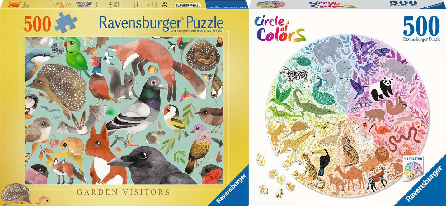
    The 2025 World Jigsaw Puzzle Championship recently took place in Spain. In the individual heats, competitors had to choose their puzzle. Each competitor could either complete a 500-piece rectangular puzzle or a 500-piece circular puzzle. For example, in Round F, puzzlers could choose one of the following two puzzles:

    There are many things to consider when picking a puzzle. First, the puzzles had already been released. This meant a puzzler could get an advantage by choosing to do a puzzle they had already completed. The image on the puzzle is also important, as is the puzzle’s style. In the example above, most puzzlers picked the circular puzzle because it had a clear colour gradient and distinct sections.

    The commentators mentioned that puzzlers might also consider the number of edge pieces. The circular puzzles have fewer edge pieces than the rectangular puzzles. This could make the rectangular puzzle easier because some puzzlers like to do the edge first and then build inwards.

    The difference in edge pieces isn’t a coincidence. Circular puzzles have fewer edge pieces than any other 500-piece puzzle. This fact is a consequence of a piece of mathematics called the isoperimetric inequality.

    The isopermetric inequality

    The isoperimetric inequality is a statement about 2D shapes. The word ‘isoperimetric’ literally translates to ‘having the same perimeter.’ The isoperimetric inequality says that if a shape has the same perimeter as a particular circle, then the circle has a larger (or equal) area. For example, the square and circle below have the same perimeter but the circle has a larger area:

    The isoperimetric inequality can also be flipped around to give a statement about shapes with the same area. This ‘having the same area’ inequality states that if a shape has the same area as a circle, then the circle has a smaller (or equal) perimeter. For example, the square and circle below have the same area but the circle has a smaller perimeter:

    The ‘having the same area’ inequality applies to the jigsaw puzzles above. In a jigsaw puzzle, the area is proportional to the number of pieces and the perimeter is proportional to the number of edge pieces (assuming the pieces are all roughly the same size and shape). This means that if one puzzle has the same number of pieces as a circular puzzle (for example 500), then the circular puzzle will have fewer edge pieces! This is exactly what the commentator said about the puzzles in the competition!

    I don’t think many of the puzzlers thought about the isopermetric inequality when picking their puzzles. But if you ever do a circular puzzle, remember that you’re doing a puzzle with as few edge pieces as possible!

  • The Multivariate Hypergeometric Distribution

    The hypergeometric distribution describes the number of white balls in a sample of \(n\) balls draw without replacement from an urn with \(m_W\) white balls and \(m_B\) black balls. The probability of having \(x\) white balls in the sample is:

    \(\displaystyle{f(x; m_W, m_B, n) = \frac{\binom{m_W}{x} \binom{m_B}{n-x}}{\binom{m_W+m_B}{n}}}\)

    This is because there are \(\binom{m_W+m_B}{n}\) possible ways to sample \(n\) balls from the urn which has \(m_W+m_B\) black balls in total. Of these possibilities, there are \(\binom{m_W}{x} \binom{m_B}{n-x}\) ways of selecting exactly \(x\) white balls.

    The multivariate hypergeometric distribution is a generalization of the hypergeometric distribution. In the multivariate hypergeometric distribution, there are \(k\) colours instead of \(2\). Suppose that the urn contains \(m_1\) balls of the first colour, \(m_2\) balls of the second colour and so on. The total number of balls in the urn is \(M = m_1+m_2+\cdots + m_k\). Next we draw \(n\) balls from the urn. Let \(X_i\) be the number of balls of colour \(i\) in our sample. The vector \(X=(X_1,X_2,\ldots, X_k)\) follows the multivariate hypergeometric distribution. The vector \(X\) satisfies the constraints \(X_i \in \{0,1,\ldots,M_i\}\) and \(\sum_{i=1}^k X_i = n\). The probability of observing \(X=x\) is

    \(\displaystyle{f(x; m, n) = \frac{\binom{m_1}{x_1} \binom{m_2}{x_2}\cdots \binom{m_k}{x_k}}{\binom{M}{n} }, \quad x_1+x_2+\cdots+x_k = n}\)

    This is because there are \(\binom{M}{n}\) possible ways of sampling \(n\) balls from the urn that has \(M\) balls in total. Likewise, The number of ways of choosing \(x_i\) balls of colour \(m_i\) is \(\binom{m_i}{x_i}\).

    Sampling

    There are two common methods for sampling from the multivariate hypergeometric distribution. The first option is to sample \(n\) numbers from \(1,\ldots,M\) without replacement. The numbers \(1,\ldots,M\) represent the balls in the urn. We can let \(1,\ldots,m_1\) represent the numbers with colour 1, and let \(m_1+1,\ldots,m_1+m_2\) represent the numbers with colour 2 and so on. Suppose that \(Y_1,\ldots,Y_n\) is the sample of size \(n\) without replacement from \(1,\ldots,M\). Next define:

    \(\displaystyle{X_i = \#\{j : X_1+X_2+\cdots+X_{i-1} < Y_j \le X_1+X_2+\cdots+X_{i-1}+X_i\}}\)

    Then the vector \(X=(X_1,\ldots,X_k)\) will be distributed according to the multivariate hypergeometric distribution. This method of sampling has complexity on the order of \(n\log(M)\). This is because sampling a random number of size \(M\) has complexity \(\log(M)\) and we need to sample \(n\) of these numbers.

    There is a second method of sampling that is more efficient when \(n\) is large and \(k\) is small. This is a sequential method that samples each \(X_i\) from a (univariate) hypergeometric distribution. The idea is that when sampling \(X_1\) we can treat the balls of colour \(1\) as “white” and all the other colours as “black”. This means that marginally, \(X_1\) is hypergeometric with parameters \(m_W = m_1\) and \(m_B = m_2+\cdots + m_k\) and \(n = n\). Furthermore, conditional on \(X_1\), the second entry, \(X_2\), is also hypergeometric. The parameters for \(X_2\) are \(m_W = m_2\), \(m_B = m_3+\cdots+m_k\) and \(n=n-X_1\). In fact, all of the conditionals of \(X\) are hypergeometric random variables and so can sampled sequentially. The python code at the end of this post implements the sequential sampler.

    The complexity of the sequential method is bounded above by \(k\) times the complexity of sampling from the hypergeometric distribution. By using the ratio of uniform distribution this can be done in complexity on the order of \(\log(m_w+m_b)\). The overall complexity of the sequential method is therefore on the order of \(k\log(M)\) which can be much smaller than \(n\log(M)\).

    import numpy as np
    
    def multivariate_hypergeometric_sample(m, n):
        x = np.zeros_like(m)
        k = len(m)
        for i in range(k-1):
            x[i] = np.random.hypergeometric(m[i], np.sum(m[(i+1):]), n)
            n -= x[i]
        x[k-1] = n
        return x
  • The maximum of geometric random variables

    I was working on a problem involving the maximum of a collection of geometric random variables. To state the problem, let \((X_i)_{i=1}^n\) be i.i.d. geometric random variables with success probability \(p=p(n)\). Next, define \(M_n = \max\{X_i : 1 \le i \le n\}\). I wanted to know the limiting distribution of \(M_n\) as \(p \to 0\) and \(n \to \infty\). I was particularly interested in the case when \(p\) was on the order of \(1/n\).

    It turns out that this problem has a very nice solution: If \(p\to 0\) as \(n \to \infty\), then for all real numbers \(c\)

    \(\displaystyle{\lim_{n \to \infty}\mathbb{P}\left(M_n \le \frac{\log n}{p}+\frac{c}{p}\right) \to \exp(-e^{-c})}\)

    That is, \(M_n\) is on the order of \(\frac{\log n}{p}\) and has fluctuations of order \(1/p\). Furthermore, these fluctuations are distributed according to the Gumbel distribution. Importantly, this result places no restrictions on how quickly \(p\) goes to \(0\).

    In the rest of this post, I’ll derive the above identity. The first step relates \(M_n\) to the maximum of a collection of exponential random variables. The second step uses a coupling to prove that the exponential and geometric random variables are close to each other.

    An easier version

    When \(p\) goes to \(0\), the scaled geometric random variables \(p X_i\) converge to exponential random variables. Exponential random variables are nicer to work because they have a continuous distribution.

    This suggests that we could try replacing all the geometric random variables with exponential random variables. More precisely, we will replace \(X_i\) with \(Y_i/p\) where \(Y_i\) are exponentially distributed. Next, we will derive the main result for the exponential random variables. Then, in the next section, we will prove that \(X_i\) is sufficiently close to \(Y_i/p\).

    Let \(\widetilde{M}_n = \max\{ Y_i/p : 1 \le i \le n\}\) where \(Y_i\) are i.i.d and exponentially distributed. This means that for \(y \ge 0\), \(\mathbb{P}(Y_i \le y)=1-e^{-y}\). The condition \(\widetilde{M}_n \le y\) is equivalent to \(Y_i \le py\) for all \(i =1,\ldots,n\). Since the \(Y_i\)’s are independent, this implies that for \(y \ge 0\)

    \(\displaystyle{\mathbb{P}(\widetilde{M}_n \le y) = \prod_{i=1}^n \mathbb{P}(Y_i \le py) = \left(1-e^{-py}\right)^n}\)

    Now fix a real number \(c\) and let \(y = \frac{\log n}{p}+\frac{c}{p}\). Since \(n \to \infty\), we know that \(y \ge 0\) for large enough \(n\). Thus, for sufficiently large \(n\)

    \(\displaystyle{\mathbb{P}\left(\widetilde{M}_n \le \frac{\log n}{p}+\frac{c}{p}\right) = \left(1-e^{-\log n – c})\right)^n = \left(1-\frac{e^{-c}}{n}\right)^n\to \exp(-e^{-c})}\)

    And so the main result holds for \(\widetilde{M}_n = \max\{Y_i/p : 1 \le i \le n\}\). We want to show that it holds for \(M_n = \max\{X_i : 1 \le i \le n\}\). The next section proves a close relationship between \(X_i\) and \(Y_i\).

    Exponential and geometric coupling

    It is true that as \(p \to 0\), \(pX_i\) converges in distribution to an exponential random variable. This is a result that holds for a single random variable. For an approximation like \(M_n \approx \widetilde{M}_n\), we need a result that works for every \(X_i\) at once. This seems tricky since it involves the convergence of an infinite collection of random variables. Fortunately, there is a simple approach based on coupling.

    For each geometric random variable \(X_i\) it is possible to produce an exponential random variables \(Y_i\) with

    \(\displaystyle{\frac{1}{\lambda} Y_i \le X_i \le \frac{1}{\lambda} Y_i + 1},\)

    where \(\lambda = -\log(1-p)\). This is because \(\mathbb{P}(X_i \le x) = 1-(1-p)^{[x]}\) and \(\mathbb{P}(Y_i/\lambda \le x) = 1-e^{-x/\lambda} = 1-(1-p)^{x}\). This means that

    \( \displaystyle{\mathbb{P}(Y_i/\lambda \le x-1) \le \mathbb{P}(X_i \le x)\le \mathbb{P}(Y_i/\lambda \le x-1) }.\)

    If we sample both \(X_i\) and \(Y_i\) with inverse transform sampling, and use the same uniform random variables, then we will have

    \(\displaystyle{ \frac{1}{\lambda} Y_i \le X_i \le \frac{1}{\lambda} Y_i + 1},\)

    as claimed. If we use this inequality for every single pair \((X_i,Y_i)\) we will get

    \(\displaystyle{\max\{Y_i/ \lambda\} \le M_n \le \max\{Y_i/\lambda\} +1}\)

    As \(p \to 0\), we have that \(\lambda \to 0\) and \(\frac{p}{\lambda}=\frac{p}{-\log(1-p)} \to 1\). This means that the random variable \(\max\{Y_i/\lambda\} \) has the same limit as \(\widetilde{M}_n = \max\{ Y_i/p : 1 \le i \le n\}\). Furthermore, \(\max\{Y_i/\lambda\} +1\) also has the same limit as \(\widetilde{M}_n\). Since \( M_n\) is “sandwiched” between \(\max\{Y_i/\lambda\}\) and \(\max\{Y_i/\lambda\} +1\), the result must also hold for \(M_n\). And so

    \(\displaystyle{\lim_{n \to \infty}\mathbb{P}\left(M_n \le \frac{\log n}{p}+\frac{c}{p}\right) \to \exp(-e^{-c})}\)

  • Uniformly sampling orthogonal matrices

    An \(n \times n\) matrix \(M \in \mathbb{R}^{n \times n}\) is orthogonal if \(M^\top M = I\). The set of all \(n \times n\) orthogonal matrices is a compact group written as \(O_n\). The uniform distribution on \(O_n\) is called Haar measure. There are many ways to generate random matrices for Haar measure. One of which is based on the Gram-Schmidt algorithm.

    Proposition. Let \(X\) be a \(n \times n\) matrix such that each entry \(X_{ij}\) is an independent standard normal random variable. Let \(x_1,x_2,\ldots,x_n \in \mathbb{R}^n\) be the columns of \(X\) and let \(q_1,q_2,\ldots,q_n \in \mathbb{R}^n\) be the result of applying Gram-Schmidt to \(x_1,x_2,\ldots,x_n\). Then the matrix \(M=[q_1,q_2,\ldots,q_n] \in O_n\) is distributed according to Haar measure.

    Another way of stating the above proposition is that if \(X\) has i.i.d. standard normal entries, and \(Q,R\) is a QR-factorization of \(X\) calculated using Gram-Schmidt, then \(Q \in O_n\) is distributed according to Haar measure. However, most numerical libraries do not use Gram-Schmidt to calculate the QR-factorization of a matrix. This means that if you generate a random \(X\) and then use your computer’s QR-factorization function, then the result might not be Haar distributed as the plot below shows.

    The plot shows an estimate of the distribution of \(\sqrt{n}M_{11}\), the top-left entry of a matrix \(M\). When \(M\) is correctly sampled, the distribution is symmetric about 0. When \(M\) is incorrectly sampled the distribution is clearly biased towards negative numbers.

    Fortunately there is a fix described in [1]! We can first use any QR-factorization algorithm to produce \(Q,R\) with \(X=QR\). We then compute a diagonal matrix \(L\) with \(L_{ii} = \mathrm{Sign}(R_{ii})\). Then, the matrix \(M=QL\) is Haar distributed. The following python code thus samples a Haar distributed matrix in \(O_n\).

    import numpy as np

    def sample_M(n):
    M = np.random.randn(n, n)
    Q, R = np.linalg.qr(M)
    L = np.sign(np.diag(R))
    return Q*L[None,:]

    References

    [1] Mezzadri, Francesco. “How to generate random matrices from the classical compact groups.” arXiv preprint math-ph/0609050 (2006). https://arxiv.org/abs/math-ph/0609050

    I recently gave a talk at the Stanford student probability seminar on Haar distributed random matrices. My notes and many further references are available here.

  • Fibonacci series

    In “Probabilizing Fibonacci Numbers” Persi Diaconis recalls asking Ron Graham to help him make his undergraduate number theory class more fun. Persi asks about the chance a Fibonacci number is even and whether infinitely many Fibonacci numbers are prime. After answering “1/3” and “no one knows” to Persi’s questions, Ron suggests giving the undergrads the following problem:

    \( \displaystyle{\sum_{n=1}^\infty \frac{F_n}{10^n} = \frac{10}{89}}\)

    While no longer an undergrad, I found the problem fun to solve and wanted to work out the general pattern. Above \(F_n\) is the \(n\)th Fibonacci number. So \(F_0=0,F_1=1\) and \(F_{n} = F_{n-1} + F_{n-2}\) for \(n \ge 2\). Ron’s infinite series can be proved using the recurrence relation for the Fibonacci numbers and the general result is that for any \(c > \varphi = \frac{1+\sqrt{5}}{2} \approx 1.618\)

    \(\displaystyle{\sum_{n=1}^\infty \frac{F_n}{c^n} = \frac{c}{c^2-c-1}}.\)

    To see why, first note that \(F_n \approx \varphi^n/\sqrt{5}\) so the sum does converge for \(c>\varphi\). Let \(x = \sum_{n=1}^\infty \frac{F_n}{c^n}\) be the value of the sum. If we multiply \(x\) by \(c^2\), then we get

    \(\displaystyle{c^2 x = \frac{c^2F_1}{c} + \sum_{n=2}^\infty \frac{F_n}{c^{n-2}} = c + \sum_{n=2}^\infty \frac{F_{n-1}}{c^{n-2}} + \sum_{n=2}^\infty \frac{F_{n-2}}{c^{n-2}} .}\)

    But

    \(\displaystyle{\sum_{n=2}^\infty \frac{F_{n-2}}{c^{n-2}}=x}\) and \(\displaystyle{\sum_{n=2}^\infty \frac{F_{n-1}}{c^{n-2}}=cx}\).

    Together this implies that \(c^2 x = c+cx+x\) and so

    \(\displaystyle{\sum_{n=1}^\infty \frac{F_n}{c^n} = x = \frac{c}{c^2-c-1}.}\)

    Generating functions

    The above calculation is closely related to the generating function of the Fibonacci numbers. The generating function of the Fibonacci numbers is the function \(f(z)\) given by

    \(\displaystyle{f(z) = \sum_{n=1}^\infty F_n z^n.}\)

    If we let \(z = c^{-1}\), then by Ron’s exercise

    \(\displaystyle{f(z) = \frac{c}{c^2-c-1}=\frac{z^{-1}}{z^{-2}-z^{-1}-1} = \frac{z}{1-z-z^2},}\)

    for \(z < \varphi^{-1}\). So solving Ron’s exercise is equivalent to finding the generating function of the Fibonacci numbers!

    Other sums

    In “Probabilizing Fibonacci Numbers”, Ron also suggests getting the undergrads to add up \(\sum_{k=0}^\infty \frac{1}{F_{2^k}}\). I leave this sum for another blog post!