Suppose we have independent events \(E_1,E_2,\ldots,E_m\), each of which occur with probability \(1-\varepsilon\). The event that all of the \(E_i\) occur is \(E = \bigcap_{i=1}^m E_i\). By using independence we can calculate the probability of \(E\),
We can therefore conclude that \((1-\varepsilon)^m \ge 1-m\varepsilon\). This is an instance of Bernoulli’s inequality. More generally, Bernoulli’s inequality states that
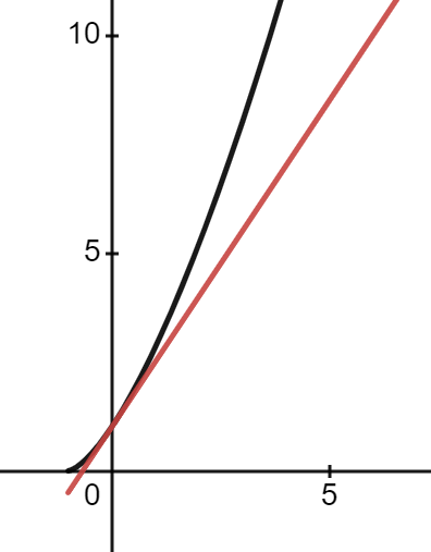
\((1+x)^m \ge 1+mx,\)
for all \(x \ge -1\) and \(m \ge 1\). This inequality states the red line is always underneath the black curve in the below picture. For an interactive version of this graph where you can change the value of \(m\), click here.
Our probabilistic proof only applies to that case when \(x = -\varepsilon\) is between \(-1\) and \(0\) and \(m\) is an integer. The more general result can be proved by using convexity. For \(m \ge 1\), the function \(f(x) = (1+x)^m\) is convex on the set \(x > -1\). The function \(g(x) = 1+mx\) is the tangent line of this function at the point \(x=0\). Convexity of \(f(x)\) means that the graph of \(f(x)\) is always above the tangent line \(g(x)\). This tells us that \((1+x)^m \ge 1+mx\).
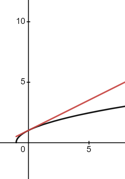
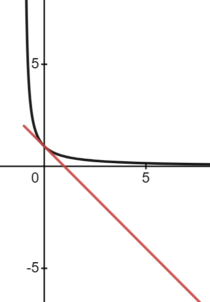
For \(m\) between \(0\) and \(1\), the function \((1+x)^m\) is no longer convex but actually concave and the inequality reverses. For \(m \le 0\), \((1+x)^m\) becomes concave again. These two cases are visualized below. In the first picture \(m = 0.5\) and the red line is above the black one. In the second picture \(m = -1\) and the black line is back on top.
Next week I’ll be starting the second year of my statistics PhD. I’ve learnt a lot from taking the first year classes and studying for the qualifying exams. Some of what I’ve learnt has given me a new perspective on some of my old blog posts. Here are three things that I’ve written about before and I now understand better.
1. The Pi-Lambda Theorem
An early post on this blog was titled “A minimal counterexample in probability theory“. The post was about a theorem from the probability course offered at the Australian National University. The theorem states that if two probability measures agree on a collection of subsets and the collection is closed under finite intersections, then the two probability measures agree on the \(\sigma\)-algebra generated by the collection. In my post I give an example which shows that you need the collection to be closed under finite intersections. I also show that you need to have at least four points in the space to find such an example.
What I didn’t know then is that the above theorem is really a corollary of Dykin’s \(\pi – \lambda\) theorem. This theorem was proved in my first graduate probability course which was taught by Persi Diaconis. Professor Diaconis kept a running tally of how many times we used the \(\pi – \lambda\) theorem in his course and we got up to at least 10. (For more appearances by Professor Diaconis on this blog see here, here and here).
If I were to write the above post again, I would talk about the \(\pi – \lambda\) theorem and rename the post “The smallest \(\lambda\)-system”. The example given in my post is really about needing at least four points to find a \(\lambda\)-system that is not a \(\sigma\)-algebra.
2. Mallow’s Cp statistic
The very first blog post I wrote was called “Complexity Penalties in Statistical Learning“. I wasn’t sure if I would write a second and so I didn’t set up a WordPress account. I instead put the post on the website LessWrong. I no longer associate myself with the rationality community but posting to LessWrong was straight forward and helped me reach more people.
The post was inspired in two ways by the 2019 AMSI summer school. First, the content is from the statistical learning course I took at the summer school. Second, at the career fair many employers advised us to work on our writing skills. I don’t know if would have started blogging if not for the AMSI Summer School.
I didn’t know it at the time but the blog post is really about Mallow’s Cp statistic. Mallow’s Cp statistic is an estimate of the test error of a regression model fit using ordinary least squares. The Mallow’s Cp is equal to the training error plus a “complexity penalty” which takes into account the number of parameters. In the blog post I talk about model complexity and over-fitting. I also write down and explain Mallow’s Cp in the special case of polynomial regression.
In the summer school course I took, I don’t remember the name Mallow’s Cp being used but I thought it was a great idea and enjoyed writing about it. The next time encountered Mallow’s Cp was in the linear models course I took last fall. I was delighted to see it again and learn how it fit into a bigger picture. More recently, I read Brad Efron’s paper “How Biased is the Apparent Error Rate of a Prediction Rule?“. The paper introduces the idea of “effective degrees of freedom” and expands on the ideas behind the Cp statistic.
Incidentally, enrolment is now open for the 2023 AMSI Summer School! This summer it will be hosted at the University of Melbourne. I encourage any Australia mathematics or statistics students reading this to take a look and apply. I really enjoyed going in both 2019 and 2020. (Also if you click on the above link you can try to spot me in the group photo of everyone wearing read shirts!)
3. Finitely additive probability measures
In “Finitely additive measures” I talk about how hard it is to define a finitely additive measure on the set of natural numbers that is not countably additive. In particular, I talked about needing to use the Hahn — Banach extension theorem to extend the natural density from the collection of sets with density to the collection of all subsets of the natural numbers.
There were a number of homework problems in my first graduate probability course that relate to this post. We proved that the sets with density are not closed under finite unions and we showed that the square free numbers have density \(6/\pi^2\).
We also proved that any finite measure defined on an algebra of subsets can be extend to the collection of all subsets. This proof used Zorn’s lemma and the resulting measure is far from unique. The use of Zorn’s lemma relates to the main idea in my blog, that defining an additive probability measure is in some sense non-constructive.
Other posts
Going forward, I hope to continue publishing at least one new post every month. I look forward to one day writing another post like this when I can look back and reflect on how much I have learnt.
The material was based on the discussion and references given in this stackexchange post. The title is a reference to a Halloween lecture on measurability given by Professor Persi Diaconis.
What’s scarier than a non-measurable set?
Making every set measurable. Or rather one particular consequence of making every set measurable.
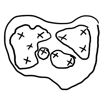
In my talk, I argued that if you make every set measurable, then there exists a set \(\Omega\) and an equivalence relation \(\sim\) on \(\Omega\) such that \(|\Omega| < |\Omega / \sim|\). That is, the set \(\Omega\) has strictly smaller cardinality than the set of equivalence classes \(\Omega/\sim\). The contradictory nature of this statement is illustrated in the picture below
We can think of the set \(\Omega\) as the collection of crosses drawn above. The equivalence relation \(\sim\) divides \(\Omega\) into the regions drawn above. The statement \(|\Omega|<|\Omega /\sim|\) means that in some sense there are more regions than crosses.
To make sense of this we’ll first have to be a bit more precise about what we mean by cardinality.
What do we mean by bigger and smaller?
Let \(A\) and \(B\) be two sets. We say that \(A\) and \(B\) have the same cardinality and write \(|A| = |B|\) if there exists a bijection function \(f:A \to B\). We can think of the function \(f\) as a way of pairing each element of \(A\) with a unique element of \(B\) such that every element of \(B\) is paired with an element of \(A\).
We next want to define \(|A|\le |B|\) which means \(A\) has cardinality at most the cardinality of \(B\). There are two reasonable ways in which we could try to define this relationship
We could say \(|A|\le |B|\) means that there exists an injective function \(f : A \to B\).
Alternatively, we could \(|A|\le |B|\) means that there exists a surjective function \(g:B \to A\).
Definitions 1 and 2 say similar things and, in the presence of the axiom of choice, they are equivalent. Since we are going to be making every set measurable in this talk, we won’t be assuming the axiom of choice. Definitions 1 and 2 are thus no longer equivalent and we have a decision to make. We will use definition . in this talk. For justification, note that definition 1 implies that there exists a subset \(B’ \subseteq B\) such that \(|A|=|B|\). We simply take \(B’\) to be the range of \(f\). This is a desirable property of the relation \(|A|\le |B|\) and it’s not clear how this could be done using definition 2.
Infinite binary sequences
It’s time to introduce the set \(\Omega\) and the equivalence relation we will be working with. The set \(\Omega\) is the set \(\{0,1\}^\mathbb{Z}\) the set of all function \(\omega : \mathbb{Z} \to \{0,1\}\). We can think of each elements \(\omega \in \Omega\) as an infinite sequence of zeros and ones stretching off in both directions. For example
\(\omega = \ldots 1110110100111\ldots\).
But this analogy hides something important. Each \(\omega \in \Omega\) has a “middle” which is the point \(\omega_0\). For instance, the two sequences below look the same but when we make \(\omega_0\) bold we see that they are different.
The equivalence relation \(\sim\) on \(\Omega\) can be thought of as forgetting the location \(\omega_0\). More formally we have \(\omega \sim \omega’\) if and only if there exists \(n \in \mathbb{Z}\) such that \(\omega_{n+k} = \omega_{k}’\) for all \(k \in \mathbb{Z}\). That is, if we shift the sequence \(\omega\) by \(n\) we get the sequence \(\omega’\). We will use \([\omega]\) to denote the equivalence class of \(\omega\) and \(\Omega/\sim\) for the set of all equivalences classes.
Some probability
Associated with the space \(\Omega\) are functions \(X_k : \Omega \to \{0,1\}\), one for each integer \(k \in \mathbb{Z}\). These functions simply evaluate \(\omega\) at \(k\). That is \(X_k(\omega)=\omega_k\). A probabilist or statistician would think of \(X_k\) as reporting the result of one of infinitely many independent coin tosses. Normally to make this formal we would have to first define a \(\sigma\)-algebra on \(\Omega\) and then define a probability on this \(\sigma\)-algebra. Today we’re working in a world where every set is measurable and so don’t have to worry about \(\sigma\)-algebras. Indeed we have the following result:
(Solovay, 1970)1There exists a model of the Zermelo Fraenkel axioms of set theory such that there exists a probability \(\mathbb{P}\) defined on all subsets of \(\Omega\) such that \(X_k\) are i.i.d. \(\mathrm{Bernoulli}(0.5)\).
This result is saying that there is world in which, other than the axiom of choice, all the regular axioms of set theory holds. And in this world, we can assign a probability to every subset \(A \subseteq \Omega\) in a way so that the events \( \{X_k=1\}\) are all independent and have probability \(0.5\). It’s important to note that this is a true countably additive probability and we can apply all our familiar probability results to \(\mathbb{P}\). We are now ready to state and prove the spooky result claimed at the start of this talk.
Proposition: Given the existence of such a probability \(\mathbb{P}\), \(|\Omega | < |\Omega /\sim|\).
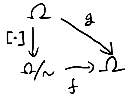
Proof: Let \(f:\Omega/\sim \to \Omega\) be any function. To show that \(|\Omega|<|\Omega /\sim|\) we need to show that \(f\) is not injective. To do this, we’ll first define another function \(g:\Omega \to \Omega\) given by \(g(\omega)=f([\omega])\). That is, \(g\) first maps \(\omega\) to \(\omega\)’s equivalence class and then applies \(f\) to this equivalence class. This is illustrated below.
A commutative diagram showing the definition of \(g\) as \(g(\omega)=f([\omega])\).
We will show that \(g : \Omega \to \Omega\) is almost surely constant with respect to \(\mathbb{P}\). That is, there exists \(\omega^\star \in \Omega\) such that \(\mathbb{P}(g(\omega)=\omega^\star)=1\). Each equivalence class \([\omega]\) is finite or countable and thus has probability zero under \(\mathbb{P}\). This means that if \(g\) is almost surely constant, then \(f\) cannot be injective and must map multiple (in fact infinitely many) equivalence classes to \(\omega^\star\).
It thus remains to show that \(g:\Omega \to \Omega\) is almost surely constant. To do this we will introduce a third function \(\varphi : \Omega \to \Omega\). The map \(\varphi\) is simply the shift map and is given by \(\varphi(\omega)_k = \omega_{k+1}\). Note that \(\omega\) and \(\varphi(\omega)\) are in the same equivalence class for every \(\omega\in \Omega\). Thus, the map \(g\) satisfies \(g\circ \varphi = g\). That is \(g\) is \(\varphi\)-invariant.
The map \(\varphi\) is ergodic. This means that if \(A \subseteq \Omega\) satisfies \(\varphi(A)=A\), then \(\mathbb{P}(A)\) equals \(0\) or \(1\). For example if \(A\) is the event that \(10110\) appears at some point in \(\omega\), then \(\varphi(A)=A\) and \(\mathbb{P}(A)=`1\). Likewise if \(A\) is the event that the relative frequency of heads converges to a number strictly greater than \(0.5\), then \(\varphi(A)=A\) and \(\mathbb{P}(A)=0\). The general claim that all \(\varphi\)-invariant events have probability \(0\) or \(1\) can be proved using the independence of \(X_k\).
For each \(k\), define an event \(A_k\) by \(A_k = \{\omega : g(\omega)_k = 1\}\). Since \(g\) is \(\varphi\)-invariant we have that \(\varphi(A_k)=A_k\). Thus, \(\mathbb{P}(A_k)=0\) or \(1\). This gives us a function \(\omega^\star :\mathbb{Z} \to \{0,1\}\) given by \(\omega^\star_k = \mathbb{P}(A_k)\). Note that for every \(k\), \(\mathbb{P}(\{\omega : g(\omega)_k = \omega_k^\star\}) = 1\). This is because if \(w_{k}^\star=1\), then \(\mathbb{P}(\{\omega: g(\omega)_k = 1\})=1\), by definition of \(w_k^\star\). Likewise if \(\omega_k^\star =0\), then \(\mathbb{P}(\{\omega:g(\omega)_k=1\})=0\) and hence \(\mathbb{P}(\{\omega:g(\omega)_k=0\})=1\). Thus, in both cases, \(\mathbb{P}(\{\omega : g(\omega)_k = \omega_k^*\})= 1\).
Since \(\mathbb{P}\) is a probability measure, we can conclude that
Thus, \(g\) map \(\Omega\) to \(\omega^\star\) with probability one. Showing that \(g\) is almost surely constant and hence that \(f\) is not injective. \(\square\)
There’s a catch!
So we have proved that there cannot be an injective map \(f : \Omega/\sim \to \Omega\). Does this mean we have proved \(|\Omega| < |\Omega/\sim|\)? Technically no. We have proved the negation of \(|\Omega/\sim|\le |\Omega|\) which does not imply \(|\Omega| \le |\Omega/\sim|\). To argue that \(|\Omega| < |\Omega/\sim|\) we need to produce a map \(g: \Omega \to \Omega/\sim\) that is injective. Surprising this is possible and not too difficult. The idea is to find a map \(g : \Omega \to \Omega\) such that \(g(\omega)\sim g(\omega’)\) implies that \(\omega = \omega’\). This can be done by somehow encoding in \(g(\omega)\) where the centre of \(\omega\) is.
A simpler proof and other examples
Our proof was nice because we explicitly calculated the value \(\omega^\star\) where \(g\) sent almost all of \(\Omega\). We could have been less explicit and simply noted that the function \(g:\Omega \to \Omega\) was measurable with respect to the invariant \(\sigma\)-algebra of \(\varphi\) and hence almost surely constant by the ergodicity of \(\varphi\).
This quicker proof allows us to generalise our “spooky result” to other sets. Below are two examples where \(\Omega = [0,1)\)
Fix \(\theta \in [0,1)\setminus \mathbb{Q}\) and define \(\omega \sim \omega’\) if and only if \(\omega + n \theta= \omega’\) for some \(n \in \mathbb{Z}\).
\(\omega \sim \omega’\) if and only if \(\omega – \omega’ \in \mathbb{Q}\).
A similar argument can be used to show that in Solovay’s world \(|\Omega| < |\Omega/\sim|\). The exact same argument follows from the ergodicity of the corresponding actions on \(\Omega\) under the uniform measure.
Three takeaways
I hope you agree that this example is good fun and surprising. I’d like to end with some remarks.
The first remark is some mathematical context. This argument given today is linked to some interesting mathematics called descriptive set theory. This field studies the properties of well behaved subsets (such as Borel subsets) of topological spaces. Descriptive set theory incorporates logic, topology and ergodic theory. I don’t know much about the field but in Persi’s Halloween talk he said that one “monster” was that few people are interested in the subject.
The next remark is a better way to think about our “spooky result”. The result is really saying something about cardinality. When we no longer use the axiom of choice, cardinality becomes a subtle concept. The statement \(|A|\le |B|\) no longer corresponds to \(A\) being “smaller” than \(B\) but rather that \(A\) is “less complex” than \(B\). This is perhaps analogous to some statistical models which may be “large” but do not overfit due to subtle constraints on the model complexity.
In light of the previous remark, I would invite you to think about whether the example I gave is truly spookier than non-measurable sets. It might seem to you that it is simply a reasonable consequence of removing the axiom of choice and restricting ourselves to functions we could actually write down or understand. I’ll let you decide
Footnotes
Technically Solovay proved that there exists a model of set theory such that every subset of \(\mathbb{R}\) is Borel measurable. To get the result for binary sequences we have to restrict to \([0,1)\) and use the binary expansion of \(x \in [0,1)\) to define a function \([0,1) \to \Omega\). Solvay’s paper is available here https://www.jstor.org/stable/1970696?seq=1
Something very exciting this afternoon. Professor Persi Diaconis was presenting at the Stanford probability seminar and the field with one element made an appearance. The talk was about joint work with Mackenzie Simper and Arun Ram. They had developed a way of “collapsing” a random walk on a group to a random walk on the set of double cosets. As an illustrative example, Persi discussed a random walk on \(GL_n(\mathbb{F}_q)\) given by multiplication by a random transvection (a map of the form \(v \mapsto v + ab^Tv\), where \(a^Tb = 0\)).
The Bruhat decomposition can be used to match double cosets of \(GL_n(\mathbb{F}_q)\) with elements of the symmetric group \(S_n\). So by collapsing the random walk on \(GL_n(\mathbb{F}_q)\) we get a random walk on \(S_n\) for all prime powers \(q\). As Professor Diaconis said, you can’t stop him from taking \(q \to 1\) and asking what the resulting random walk on \(S_n\) is. The answer? Multiplication by a random transposition. As pointed sets are vector spaces over the field with one element and the symmetric groups are the matrix groups, this all fits with what’s expected of the field with one element.
This was just one small part of a very enjoyable seminar. There was plenty of group theory, probability, some general theory and engaging examples.
Update: I have written another post about some of the group theory from the seminar! You can read it here: Double cosets and contingency tables.
It is winter 2022 and my PhD cohort has moved on the second quarter of our first year statistics courses. This means we’ll be learning about generalised linear models in our applied course, asymptotic statistics in our theory course and conditional expectations and martingales in our probability course.
In the first week of our probability course we’ve been busy defining and proving the existence of the conditional expectation. Our approach has been similar to how we constructed the Lebesgue integral in the previous course. Last quarter, we first defined the Lebesgue integral for simple functions, then we used a limiting argument to define the Lebesgue integral for non-negative functions and then finally we defined the Lebesgue integral for arbitrary functions by considering their positive and negative parts.
Our approach to the conditional expectation has been similar but the journey has been different. We again started with simple random variables, then progressed to non-negative random variables and then proved the existence of the conditional expectation of any arbitrary integrable random variable. Unlike the Lebesgue integral, the hardest step was proving the existence of the conditional expectation of a simple random variable. Progressing from simple random variables to arbitrary random variables was a straight forward application of the monotone convergence theorem and linearity of expectation. But to prove the existence of the conditional expectation of a simple random variable we needed to work with projections in the Hilbert space \(L^2(\Omega, \mathbb{P},\mathcal{F})\).
Unlike the Lebesgue integral, defining the conditional expectation of a simple random variable is not straight forward. One reason for this is that the conditional expectation of a random variable need not be a simple random variable. This comment was made off hand by our Professor and sparked my curiosity. The following example is what I came up with. Below I first go over some definitions and then we dive into the example.
A simple random variable with a conditional expectation that is not simple
Let \((\Omega, \mathbb{P}, \mathcal{F})\) be a probability space and let \(\mathcal{G} \subseteq \mathcal{F}\) be a sub-\(\sigma\)-algebra. The conditional expectation of an integrable random variable \(X\) is a random variable \(\mathbb{E}(X|\mathcal{G})\) that satisfies the following two conditions:
The random variable \(\mathbb{E}(X|\mathcal{G})\) is \(\mathcal{G}\)-measurable.
For all \(B \in \mathcal{G}\), \(\mathbb{E}[X1_B] = \mathbb{E}[\mathbb{E}(X|\mathcal{G})1_B]\), where \(1_B\) is the indicator function of \(B\).
The conditional expectation of an integrable random variable is unique and always exists. One can think of \(\mathbb{E}(X|\mathcal{G})\) as the expected value of \(X\) given the information in \(\mathcal{G}\).
A simple random variable is a random variable \(X\) that take only finitely many values. Simple random variables are always integrable and so \(\mathbb{E}(X|\mathcal{G})\) always exists but we will see that \(\mathbb{E}(X|\mathcal{G})\) need not be simple.
Consider a random vector \((U,V)\) uniformly distributed on the square \([-1,1]^2 \subseteq \mathbb{R}^2\). Let \(D\) be the unit disc \(D = \{(u,v) \in \mathbb{R}^2:u^2+v^2 \le 1\}\). The random variable \(X = 1_D(U,V)\) is a simple random variable since \(X\) equals \(1\) if \((U,V) \in D\) and \(X\) equals \(0\) otherwise. Let \(\mathcal{G} = \sigma(U)\) the \(\sigma\)-algebra generated by \(U\). It turns out that
\(\mathbb{E}(X|\mathcal{G}) = \sqrt{1-U^2}\).
Thus \(\mathbb{E}(X|\mathcal{G})\) is not a simple random variable. Let \(Y = \sqrt{1-U^2}\). Since \(Y\) is a continuous function of \(U\), the random variable is \(\mathcal{G}\)-measurable. Thus \(Y\) satisfies condition 1. Furthermore if \(B \in \mathcal{G}\), then \(B = \{U \in A\}\) for some measurable set \(A\subseteq [-1,1]\). Thus \(X1_B\) equals \(1\) if and only if \(U \in A\) and \(V \in [-\sqrt{1-U^2}, \sqrt{1-U^2}]\). Since \((U,V)\) is uniformly distributed we thus have
Thus \(\mathbb{E}[X1_B] = \mathbb{E}[Y1_B]\) and therefore \(Y = \sqrt{1-U^2}\) equals \(\mathbb{E}(X|\mathcal{G})\). Intuitively we can see this because given \(U=u\), we know that \(X\) is \(1\) when \(V \in [-\sqrt{1-u^2},\sqrt{1+u^2}]\) and that \(X\) is \(0\) otherwise. Since \(V\) is uniformly distributed on \([-1,1]\) the probability that \(V\) is in \([-\sqrt{1-u^2},\sqrt{1+u^2}]\) is \(\sqrt{1-u^2}\). Thus given \(U=u\), the expected value of \(X\) is \(\sqrt{1-u^2}\).
An extension
The previous example suggests an extension that shows just how “complicated” the conditional expectation of a simple random variable can be. I’ll state the extension as an exercise:
Let \(f:[-1,1]\to \mathbb{R}\) be any continuous function with \(f(x) \in [0,1]\). With \((U,V)\) and \(\mathcal{G}\) as above show that there exists a measurable set \(A \subseteq [-1,1]^2\) such that \(\mathbb{E}(1_A|\mathcal{G}) = f(U)\).