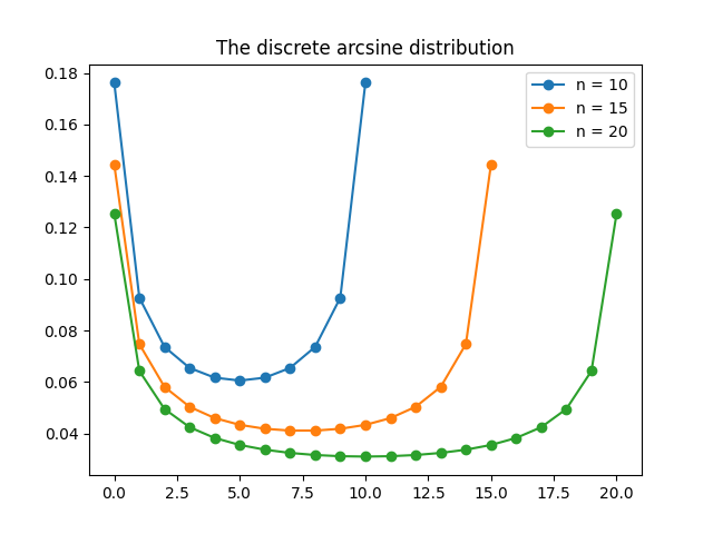
Category: Probability

  • Monte Carlo integration in high dimensions

    Monte Carlo integration

    John Cook recently wrote a cautionary blog post about using Monte Carlo to estimate the volume of a high-dimensional ball. He points out that if \(\mathbf{X}=(X_1,\ldots,X_n)\) are independent and uniformly distributed on the interval \([-1,1]\) then

    \(\displaystyle{\mathbb{P}(X_1^2 + X_2^2 + \cdots + X_n^2 \le 1) = \frac{v_n}{2^n}},\)

    where \(v_n\) is the volume of an \(n\)-dimensional ball with radius one. This observation means that we can use Monte Carlo to estimate \(v_n\).

    To do this we repeatedly sample vectors \(\mathbf{X}_m = (X_{m,1},\ldots,X_{m,n})\) with \(X_{m,i}\) uniform on \([-1,1]\) and \(m\) ranging from \(1\) to \(M\). Next, we count the proportion of vectors \(\mathbf{X}_m\) with \(X_{1,m}^2 + \cdots + X_{n,m}^2 \le 1\). Specifically, if \(Z_m\) is equal to one when \(X_{1,m}^2 + \cdots + X_{n,m}^2 \le 1\) and equal to zero otherwise, then by the law of large numbers

    \(\displaystyle{\frac{1}{M}\sum_{m=1}^M Z_m \approx \frac{v_n}{2^n}}\)

    Which implies

    \(v_n \approx 2^n \frac{1}{M}\sum_{m=1}^M Z_m\)

    This method of approximating a volume or integral by sampling and counting is called Monte Carlo integration and is a powerful general tool in scientific computing.

    The problem with Monte Carlo integration

    As pointed out by John, Monte Carlo integration does not work very well in this example. The plot below shows a large difference between the true value of \(v_n\) with \(n\) ranging from \(1\) to \(20\) and the Monte Carlo approximation with \(M = 1,000\).

    The problem is that \(v_n\) is very small and the probability \(v_n/2^n\) is even smaller! For example when \(n = 10\), \(v_n/2^n \approx 0.0025\). This means that in our one thousand samples we only expect two or three occurrences of the event \(X_{m,1}^2 + \cdots + X_{m,n}^2 \le 1\). As a result our estimate has a high variance.

    The results get even worse as \(n\) increases. The probability \(v_n/2^n\) does to zero faster than exponentially. Even with a large value of \(M\), our estimate will be zero. Since \(v_n \neq 0\), the relative error in the approximation is 100%.

    Importance sampling

    Monte Carlo can still be used to approximate \(v_n\). Instead of using plain Monte Carlo, we can use a variance reduction technique called importance sampling (IS). Instead of sampling the points \(X_{m,1},\ldots, X_{m,n}\) from the uniform distribution on \([-1,1]\), we can instead sample the from some other distribution called a proposal distribution. The proposal distribution should be chosen so that that the event \(X_{m,1}^2 +\cdots +X_{m,n}^2 \le 1\) becomes more likely.

    In importance sampling, we need to correct for the fact that we are using a new distribution instead of the uniform distribution. Instead of the counting the number of times \(X_{m,1}^2+\cdots+X_{m,n}^2 \le 1\) , we give weights to each of samples and then add up the weights.

    If \(p\) is the density of the uniform distribution on \([-1,1]\) (the target distribution) and \(q\) is the density of the proposal distribution, then the IS Monte Carlo estimate of \(v_n\) is

    \(\displaystyle{\frac{1}{M}\sum_{m=1}^M Z_m \prod_{i=1}^n \frac{p(X_{m,i})}{q(X_{m,i})}},\)

    where as before \(Z_m\) is one if \(X_{m,1}^2+\cdots +X_{m,n}^2 \le 1\) and \(Z_m\) is zero otherwise. As long as \(q(x)=0\) implies \(p(x)=0\), the IS Monte Carlo estimate will be an unbiased estimate of \(v_n\). More importantly, a good choice of the proposal distribution \(q\) can drastically reduce the variance of the IS estimate compared to the plain Monte Carlo estimate.

    In this example, a good choice of proposal distribution is the normal distribution with mean \(0\) and variance \(1/n\). Under this proposal distribution, the expected value of \(X_{m,1}^2 +\cdots+ X_{m,n}^2\) is one and so the event \(X_{m,1}^2 + \cdots + X_{m,n}^2 \le 1\) is much more likely.

    Here are the IS Monte Carlo estimates with again \(M = 1,000\) and \(n\) ranging from \(1\) to \(20\). The results speak for themselves.

    The relative error is typically less than 10%. A big improvement over the 100% relative error of plain Monte Carlo.

    The next plot shows a close agreement between \(v_n\) and the IS Monte Carlo approximation on the log scale with \(n\) going all the way up to \(100\).

    Notes

    1. There are exact formulas for \(v_n\) (available on Wikipedia). I used these to compare the approximations and compute relative errors. There are related problems where no formulas exist and Monte Carlo integration is one of the only ways to get an approximate answer.
    2. The post by John Cook also talks about why the central limit theorem can’t be used to approximate \(v_n\). I initially thought a technique called large deviations could be used to approximate \(v_n\) but again this does not directly apply. I was happy to discover that importance sampling worked so well!

    More sampling posts

  • Auxiliary variables sampler

    The auxiliary variables sampler is a general Markov chain Monte Carlo (MCMC) technique for sampling from probability distributions with unknown normalizing constants [1, Section 3.1]. Specifically, suppose we have \(n\) functions \(f_i : \mathcal{X} \to (0,\infty)\) and we want to sample from the probability distribution \(P(x) \propto \prod_{i=1}^n f_i(x).\) That is

    \(\displaystyle{ P(x) = \frac{1}{Z}\prod_{i=1}^n f_i(x)},\)

    where \(Z = \sum_{x \in \mathcal{X}} \prod_{i=1}^n f_i(x)\) is a normalizing constant. If the set \(\mathcal{X}\) is very large, then it may be difficult to compute \(Z\) or sample from \(P(x)\). To approximately sample from \(P(x)\) we can run an ergodic Markov chain with \(P(x)\) as a stationary distribution. Adding auxiliary variables is one way to create such a Markov chain. For each \(i \in \{1,\ldots,n\}\), we add a auxiliary variable \(U_i \ge 0\) such that

    \(\displaystyle{P(U \mid X) = \prod_{i=1}^n \mathrm{Unif}[0,f_i(X)]}.\)

    That is, conditional on \(X\), the auxiliary variables \(U_1,\ldots,U_n\) are independent and \(U_i\) is uniformly distributed on the interval \([0,f_i(X)]\). If \(X\) is distributed according to \(P\) and \(U_1,\ldots,U_n\) have the above auxiliary variable distribution, then

    \(\displaystyle{P(X,U) =P(X)P(U\mid X)\propto \prod_{i=1}^n f_i(X) \frac{1}{f_i(X)} I[U_i \le f(X_i)] = \prod_{i=1}^n I[U_i \le f(X_i)]}.\)

    This means that the joint distribution of \((X,U)\) is uniform on the set

    \(\widetilde{\mathcal{X}} = \{(x,u) \in \mathcal{X} \times (0,\infty)^n : u_i \le f(x_i) \text{ for all } i\}.\)

    Put another way, suppose we could jointly sample \((X,U)\) from the uniform distribution on \(\widetilde{\mathcal{X}}\). Then, the above calculation shows that if we discard \(U\) and only keep \(X\), then \(X\) will be sampled from our target distribution \(P\).

    The auxiliary variables sampler approximately samples from the uniform distribution on \(\widetilde{\mathcal{X}}\) is by using a Gibbs sampler. The Gibbs samplers alternates between sampling \(U’\) from \(P(U \mid X)\) and then sampling \(X’\) from \(P(X \mid U’)\). Since the joint distribution of \((X,U)\) is uniform on \(\widetilde{\mathcal{X}}\), the conditional distributions \(P(X \mid U)\) and \(P(U \mid X)\) are also uniform. The auxiliary variables sampler thus transitions from \(X\) to \(X’\) according to the two step process

    1. Independently sample \(U_i\) uniformly from \([0,f_i(X)]\).
    2. Sample \(X’\) uniformly from the set \(\{x \in \mathcal{X} : f_i(x) \ge u_i \text{ for all } i\}\).

    Since the auxiliary variables sampler is based on a Gibbs sampler, we know that the joint distribution of \((X,U)\) will converge to the uniform distribution on \(\mathcal{X}\). So when we discard \(U\), the distribution of \(X\) will converge to the target distribution \(P\)!

    Auxiliary variables in practice

    To perform step 2 of the auxiliary variables sampler we have to be able to sample uniformly from the sets

    \(\mathcal{X}_u = \{x \in \mathcal{X}:f_i(x) \ge u_i \text{ for all } i\}. \)

    Depending on the nature of the set \(\mathcal{X}\) and the functions \(f_i\), it might be difficult to do this. Fortunately, there are some notable examples where this step has been worked out. The very first example of auxiliary variables is the Swendsen-Wang algorithm for sampling from the Ising model [2]. In this model it is possible to sample uniformly from \(\mathcal{X}_u\). Another setting where we can sample exactly is when \(\mathcal{X}\) is the real numbers \(\mathcal{R}\) and each \(f_i\) is an increasing function of \(x\). This is explored in [3] where they apply auxiliary variables to sampling from Bayesian posteriors.

    There is an alternative to sampling exactly from the uniform distribution on \(\mathcal{X}_u\). Instead of sampling \(X’\) uniformly from \(\mathcal{X}_u\), we can run a Markov chain from the old \(X\) that has the uniform distribution as a stationary distribution. This approach leads to another special case of auxiliary variables which is called “slice sampling” [4].

    References

    [1] Andersen HC, Diaconis P. Hit and run as a unifying device. Journal de la societe francaise de statistique & revue de statistique appliquee. 2007;148(4):5-28. http://www.numdam.org/item/JSFS_2007__148_4_5_0/
    [2] Swendsen RH, Wang JS. Nonuniversal critical dynamics in Monte Carlo simulations. Physical review letters. 1987 Jan 12;58(2):86. https://journals.aps.org/prl/abstract/10.1103/PhysRevLett.58.86
    [3] Damlen P, Wakefield J, Walker S. Gibbs sampling for Bayesian non‐conjugate and hierarchical models by using auxiliary variables. Journal of the Royal Statistical Society: Series B (Statistical Methodology). 1999 Apr;61(2):331-44. https://rss.onlinelibrary.wiley.com/doi/abs/10.1111/1467-9868.00179
    [4] Neal RM. Slice sampling. The annals of statistics. 2003 Jun;31(3):705-67. https://projecteuclid.org/journals/annals-of-statistics/volume-31/issue-3/Slice-sampling/10.1214/aos/1056562461.full

  • Bernoulli’s inequality and probability

    Suppose we have independent events \(E_1,E_2,\ldots,E_m\), each of which occur with probability \(1-\varepsilon\). The event that all of the \(E_i\) occur is \(E = \bigcap_{i=1}^m E_i\). By using independence we can calculate the probability of \(E\),

    \(P(E) = P\left(\bigcap_{i=1}^m E_i\right) = \prod_{i=1}^m P(E_i) = (1-\varepsilon)^m.\)

    We could also get a lower bound on \(P(E)\) by using the union bound. This gives,

    \(P(E) = 1-P(E^c) = 1-P\left(\bigcup_{i=1}^m E_i^c\right) \ge `1-\sum_{i=1}^m P(E_i^c) = 1-m\varepsilon.\)

    We can therefore conclude that \((1-\varepsilon)^m \ge 1-m\varepsilon\). This is an instance of Bernoulli’s inequality. More generally, Bernoulli’s inequality states that

    \((1+x)^m \ge 1+mx,\)

    for all \(x \ge -1\) and \(m \ge 1\). This inequality states the red line is always underneath the black curve in the below picture. For an interactive version of this graph where you can change the value of \(m\), click here.

    Our probabilistic proof only applies to that case when \(x = -\varepsilon\) is between \(-1\) and \(0\) and \(m\) is an integer. The more general result can be proved by using convexity. For \(m \ge 1\), the function \(f(x) = (1+x)^m\) is convex on the set \(x > -1\). The function \(g(x) = 1+mx\) is the tangent line of this function at the point \(x=0\). Convexity of \(f(x)\) means that the graph of \(f(x)\) is always above the tangent line \(g(x)\). This tells us that \((1+x)^m \ge 1+mx\).

    For \(m\) between \(0\) and \(1\), the function \((1+x)^m\) is no longer convex but actually concave and the inequality reverses. For \(m \le 0\), \((1+x)^m\) becomes concave again. These two cases are visualized below. In the first picture \(m = 0.5\) and the red line is above the black one. In the second picture \(m = -1\) and the black line is back on top.

  • Looking back on the blog

    Next week I’ll be starting the second year of my statistics PhD. I’ve learnt a lot from taking the first year classes and studying for the qualifying exams. Some of what I’ve learnt has given me a new perspective on some of my old blog posts. Here are three things that I’ve written about before and I now understand better.

    1. The Pi-Lambda Theorem

    An early post on this blog was titled “A minimal counterexample in probability theory“. The post was about a theorem from the probability course offered at the Australian National University. The theorem states that if two probability measures agree on a collection of subsets and the collection is closed under finite intersections, then the two probability measures agree on the \(\sigma\)-algebra generated by the collection. In my post I give an example which shows that you need the collection to be closed under finite intersections. I also show that you need to have at least four points in the space to find such an example.

    What I didn’t know then is that the above theorem is really a corollary of Dykin’s \(\pi – \lambda\) theorem. This theorem was proved in my first graduate probability course which was taught by Persi Diaconis. Professor Diaconis kept a running tally of how many times we used the \(\pi – \lambda\) theorem in his course and we got up to at least 10. (For more appearances by Professor Diaconis on this blog see here, here and here).

    If I were to write the above post again, I would talk about the \(\pi – \lambda\) theorem and rename the post “The smallest \(\lambda\)-system”. The example given in my post is really about needing at least four points to find a \(\lambda\)-system that is not a \(\sigma\)-algebra.

    2. Mallow’s Cp statistic

    The very first blog post I wrote was called “Complexity Penalties in Statistical Learning“. I wasn’t sure if I would write a second and so I didn’t set up a WordPress account. I instead put the post on the website LessWrong. I no longer associate myself with the rationality community but posting to LessWrong was straight forward and helped me reach more people.

    The post was inspired in two ways by the 2019 AMSI summer school. First, the content is from the statistical learning course I took at the summer school. Second, at the career fair many employers advised us to work on our writing skills. I don’t know if would have started blogging if not for the AMSI Summer School.

    I didn’t know it at the time but the blog post is really about Mallow’s Cp statistic. Mallow’s Cp statistic is an estimate of the test error of a regression model fit using ordinary least squares. The Mallow’s Cp is equal to the training error plus a “complexity penalty” which takes into account the number of parameters. In the blog post I talk about model complexity and over-fitting. I also write down and explain Mallow’s Cp in the special case of polynomial regression.

    In the summer school course I took, I don’t remember the name Mallow’s Cp being used but I thought it was a great idea and enjoyed writing about it. The next time encountered Mallow’s Cp was in the linear models course I took last fall. I was delighted to see it again and learn how it fit into a bigger picture. More recently, I read Brad Efron’s paper “How Biased is the Apparent Error Rate of a Prediction Rule?“. The paper introduces the idea of “effective degrees of freedom” and expands on the ideas behind the Cp statistic.

    Incidentally, enrolment is now open for the 2023 AMSI Summer School! This summer it will be hosted at the University of Melbourne. I encourage any Australia mathematics or statistics students reading this to take a look and apply. I really enjoyed going in both 2019 and 2020. (Also if you click on the above link you can try to spot me in the group photo of everyone wearing read shirts!)

    3. Finitely additive probability measures

    In “Finitely additive measures” I talk about how hard it is to define a finitely additive measure on the set of natural numbers that is not countably additive. In particular, I talked about needing to use the Hahn — Banach extension theorem to extend the natural density from the collection of sets with density to the collection of all subsets of the natural numbers.

    There were a number of homework problems in my first graduate probability course that relate to this post. We proved that the sets with density are not closed under finite unions and we showed that the square free numbers have density \(6/\pi^2\).

    We also proved that any finite measure defined on an algebra of subsets can be extend to the collection of all subsets. This proof used Zorn’s lemma and the resulting measure is far from unique. The use of Zorn’s lemma relates to the main idea in my blog, that defining an additive probability measure is in some sense non-constructive.

    Other posts

    Going forward, I hope to continue publishing at least one new post every month. I look forward to one day writing another post like this when I can look back and reflect on how much I have learnt.

  • Non-measurable sets, cardinality and the axiom of choice

    The following post is based on a talk I gave at the 2022 Stanford statistics retreat. The talk was titled “Another non-measurable monster”.

    The opening slide from my presentation. The test reads “another non-measurable monster”. There are spooky pumpkins in the background. Image from https://www.shutterstock.com/image-photo/pumpkins-graveyard-spooky-night-halloween-backdrop-1803950377

    The material was based on the discussion and references given in this stackexchange post. The title is a reference to a Halloween lecture on measurability given by Professor Persi Diaconis.

    What’s scarier than a non-measurable set?

    Making every set measurable. Or rather one particular consequence of making every set measurable.

    In my talk, I argued that if you make every set measurable, then there exists a set \(\Omega\) and an equivalence relation \(\sim\) on \(\Omega\) such that \(|\Omega| < |\Omega / \sim|\). That is, the set \(\Omega\) has strictly smaller cardinality than the set of equivalence classes \(\Omega/\sim\). The contradictory nature of this statement is illustrated in the picture below

    We can think of the set \(\Omega\) as the collection of crosses drawn above. The equivalence relation \(\sim\) divides \(\Omega\) into the regions drawn above. The statement \(|\Omega|<|\Omega /\sim|\) means that in some sense there are more regions than crosses.

    To make sense of this we’ll first have to be a bit more precise about what we mean by cardinality.

    What do we mean by bigger and smaller?

    Let \(A\) and \(B\) be two sets. We say that \(A\) and \(B\) have the same cardinality and write \(|A| = |B|\) if there exists a bijection function \(f:A \to B\). We can think of the function \(f\) as a way of pairing each element of \(A\) with a unique element of \(B\) such that every element of \(B\) is paired with an element of \(A\).

    We next want to define \(|A|\le |B|\) which means \(A\) has cardinality at most the cardinality of \(B\). There are two reasonable ways in which we could try to define this relationship

    1. We could say \(|A|\le |B|\) means that there exists an injective function \(f : A \to B\).
    2. Alternatively, we could \(|A|\le |B|\) means that there exists a surjective function \(g:B \to A\).

    Definitions 1 and 2 say similar things and, in the presence of the axiom of choice, they are equivalent. Since we are going to be making every set measurable in this talk, we won’t be assuming the axiom of choice. Definitions 1 and 2 are thus no longer equivalent and we have a decision to make. We will use definition . in this talk. For justification, note that definition 1 implies that there exists a subset \(B’ \subseteq B\) such that \(|A|=|B|\). We simply take \(B’\) to be the range of \(f\). This is a desirable property of the relation \(|A|\le |B|\) and it’s not clear how this could be done using definition 2.

    Infinite binary sequences

    It’s time to introduce the set \(\Omega\) and the equivalence relation we will be working with. The set \(\Omega\) is the set \(\{0,1\}^\mathbb{Z}\) the set of all function \(\omega : \mathbb{Z} \to \{0,1\}\). We can think of each elements \(\omega \in \Omega\) as an infinite sequence of zeros and ones stretching off in both directions. For example

    \(\omega = \ldots 1110110100111\ldots\).

    But this analogy hides something important. Each \(\omega \in \Omega\) has a “middle” which is the point \(\omega_0\). For instance, the two sequences below look the same but when we make \(\omega_0\) bold we see that they are different.

    \(\omega = \ldots 111011\mathbf{0}100111\ldots\),

    \(\omega’ = \ldots 1110110\mathbf{1}00111\ldots\).

    The equivalence relation \(\sim\) on \(\Omega\) can be thought of as forgetting the location \(\omega_0\). More formally we have \(\omega \sim \omega’\) if and only if there exists \(n \in \mathbb{Z}\) such that \(\omega_{n+k} = \omega_{k}’\) for all \(k \in \mathbb{Z}\). That is, if we shift the sequence \(\omega\) by \(n\) we get the sequence \(\omega’\). We will use \([\omega]\) to denote the equivalence class of \(\omega\) and \(\Omega/\sim\) for the set of all equivalences classes.

    Some probability

    Associated with the space \(\Omega\) are functions \(X_k : \Omega \to \{0,1\}\), one for each integer \(k \in \mathbb{Z}\). These functions simply evaluate \(\omega\) at \(k\). That is \(X_k(\omega)=\omega_k\). A probabilist or statistician would think of \(X_k\) as reporting the result of one of infinitely many independent coin tosses. Normally to make this formal we would have to first define a \(\sigma\)-algebra on \(\Omega\) and then define a probability on this \(\sigma\)-algebra. Today we’re working in a world where every set is measurable and so don’t have to worry about \(\sigma\)-algebras. Indeed we have the following result:

    (Solovay, 1970)1 There exists a model of the Zermelo Fraenkel axioms of set theory such that there exists a probability \(\mathbb{P}\) defined on all subsets of \(\Omega\) such that \(X_k\) are i.i.d. \(\mathrm{Bernoulli}(0.5)\).

    This result is saying that there is world in which, other than the axiom of choice, all the regular axioms of set theory holds. And in this world, we can assign a probability to every subset \(A \subseteq \Omega\) in a way so that the events \( \{X_k=1\}\) are all independent and have probability \(0.5\). It’s important to note that this is a true countably additive probability and we can apply all our familiar probability results to \(\mathbb{P}\). We are now ready to state and prove the spooky result claimed at the start of this talk.

    Proposition: Given the existence of such a probability \(\mathbb{P}\), \(|\Omega | < |\Omega /\sim|\).

    Proof: Let \(f:\Omega/\sim \to \Omega\) be any function. To show that \(|\Omega|<|\Omega /\sim|\) we need to show that \(f\) is not injective. To do this, we’ll first define another function \(g:\Omega \to \Omega\) given by \(g(\omega)=f([\omega])\). That is, \(g\) first maps \(\omega\) to \(\omega\)’s equivalence class and then applies \(f\) to this equivalence class. This is illustrated below.

    A commutative diagram showing the definition of \(g\) as \(g(\omega)=f([\omega])\).

    We will show that \(g : \Omega \to \Omega\) is almost surely constant with respect to \(\mathbb{P}\). That is, there exists \(\omega^\star \in \Omega\) such that \(\mathbb{P}(g(\omega)=\omega^\star)=1\). Each equivalence class \([\omega]\) is finite or countable and thus has probability zero under \(\mathbb{P}\). This means that if \(g\) is almost surely constant, then \(f\) cannot be injective and must map multiple (in fact infinitely many) equivalence classes to \(\omega^\star\).

    It thus remains to show that \(g:\Omega \to \Omega\) is almost surely constant. To do this we will introduce a third function \(\varphi : \Omega \to \Omega\). The map \(\varphi\) is simply the shift map and is given by \(\varphi(\omega)_k = \omega_{k+1}\). Note that \(\omega\) and \(\varphi(\omega)\) are in the same equivalence class for every \(\omega\in \Omega\). Thus, the map \(g\) satisfies \(g\circ \varphi = g\). That is \(g\) is \(\varphi\)-invariant.

    The map \(\varphi\) is ergodic. This means that if \(A \subseteq \Omega\) satisfies \(\varphi(A)=A\), then \(\mathbb{P}(A)\) equals \(0\) or \(1\). For example if \(A\) is the event that \(10110\) appears at some point in \(\omega\), then \(\varphi(A)=A\) and \(\mathbb{P}(A)=`1\). Likewise if \(A\) is the event that the relative frequency of heads converges to a number strictly greater than \(0.5\), then \(\varphi(A)=A\) and \(\mathbb{P}(A)=0\). The general claim that all \(\varphi\)-invariant events have probability \(0\) or \(1\) can be proved using the independence of \(X_k\).

    For each \(k\), define an event \(A_k\) by \(A_k = \{\omega : g(\omega)_k = 1\}\). Since \(g\) is \(\varphi\)-invariant we have that \(\varphi(A_k)=A_k\). Thus, \(\mathbb{P}(A_k)=0\) or \(1\). This gives us a function \(\omega^\star :\mathbb{Z} \to \{0,1\}\) given by \(\omega^\star_k = \mathbb{P}(A_k)\). Note that for every \(k\), \(\mathbb{P}(\{\omega : g(\omega)_k = \omega_k^\star\}) = 1\). This is because if \(w_{k}^\star=1\), then \(\mathbb{P}(\{\omega: g(\omega)_k = 1\})=1\), by definition of \(w_k^\star\). Likewise if \(\omega_k^\star =0\), then \(\mathbb{P}(\{\omega:g(\omega)_k=1\})=0\) and hence \(\mathbb{P}(\{\omega:g(\omega)_k=0\})=1\). Thus, in both cases, \(\mathbb{P}(\{\omega : g(\omega)_k = \omega_k^*\})= 1\).

    Since \(\mathbb{P}\) is a probability measure, we can conclude that

    \(\mathbb{P}(\{\omega : g(\omega)=\omega^\star\}) = \mathbb{P}\left(\bigcap_{k \in \mathbb{Z}} \{\omega : g(\omega)_k = \omega_k^\star\}\right)=1\).

    Thus, \(g\) map \(\Omega\) to \(\omega^\star\) with probability one. Showing that \(g\) is almost surely constant and hence that \(f\) is not injective. \(\square\)

    There’s a catch!

    So we have proved that there cannot be an injective map \(f : \Omega/\sim \to \Omega\). Does this mean we have proved \(|\Omega| < |\Omega/\sim|\)? Technically no. We have proved the negation of \(|\Omega/\sim|\le |\Omega|\) which does not imply \(|\Omega| \le |\Omega/\sim|\). To argue that \(|\Omega| < |\Omega/\sim|\) we need to produce a map \(g: \Omega \to \Omega/\sim\) that is injective. Surprising this is possible and not too difficult. The idea is to find a map \(g : \Omega \to \Omega\) such that \(g(\omega)\sim g(\omega’)\) implies that \(\omega = \omega’\). This can be done by somehow encoding in \(g(\omega)\) where the centre of \(\omega\) is.

    A simpler proof and other examples

    Our proof was nice because we explicitly calculated the value \(\omega^\star\) where \(g\) sent almost all of \(\Omega\). We could have been less explicit and simply noted that the function \(g:\Omega \to \Omega\) was measurable with respect to the invariant \(\sigma\)-algebra of \(\varphi\) and hence almost surely constant by the ergodicity of \(\varphi\).

    This quicker proof allows us to generalise our “spooky result” to other sets. Below are two examples where \(\Omega = [0,1)\)

    • Fix \(\theta \in [0,1)\setminus \mathbb{Q}\) and define \(\omega \sim \omega’\) if and only if \(\omega + n \theta= \omega’\) for some \(n \in \mathbb{Z}\).
    • \(\omega \sim \omega’\) if and only if \(\omega – \omega’ \in \mathbb{Q}\).

    A similar argument can be used to show that in Solovay’s world \(|\Omega| < |\Omega/\sim|\). The exact same argument follows from the ergodicity of the corresponding actions on \(\Omega\) under the uniform measure.

    Three takeaways

    I hope you agree that this example is good fun and surprising. I’d like to end with some remarks.

    • The first remark is some mathematical context. This argument given today is linked to some interesting mathematics called descriptive set theory. This field studies the properties of well behaved subsets (such as Borel subsets) of topological spaces. Descriptive set theory incorporates logic, topology and ergodic theory. I don’t know much about the field but in Persi’s Halloween talk he said that one “monster” was that few people are interested in the subject.
    • The next remark is a better way to think about our “spooky result”. The result is really saying something about cardinality. When we no longer use the axiom of choice, cardinality becomes a subtle concept. The statement \(|A|\le |B|\) no longer corresponds to \(A\) being “smaller” than \(B\) but rather that \(A\) is “less complex” than \(B\). This is perhaps analogous to some statistical models which may be “large” but do not overfit due to subtle constraints on the model complexity.
    • In light of the previous remark, I would invite you to think about whether the example I gave is truly spookier than non-measurable sets. It might seem to you that it is simply a reasonable consequence of removing the axiom of choice and restricting ourselves to functions we could actually write down or understand. I’ll let you decide

    Footnotes

    1. Technically Solovay proved that there exists a model of set theory such that every subset of \(\mathbb{R}\) is Borel measurable. To get the result for binary sequences we have to restrict to \([0,1)\) and use the binary expansion of \(x \in [0,1)\) to define a function \([0,1) \to \Omega\). Solvay’s paper is available here https://www.jstor.org/stable/1970696?seq=1