Category: numerical-methods

  • Poisson approximations to the negative binomial distribution

    This post is an introduction to the negative binomial distribution and a discussion of different ways of approximating the negative binomial distribution.

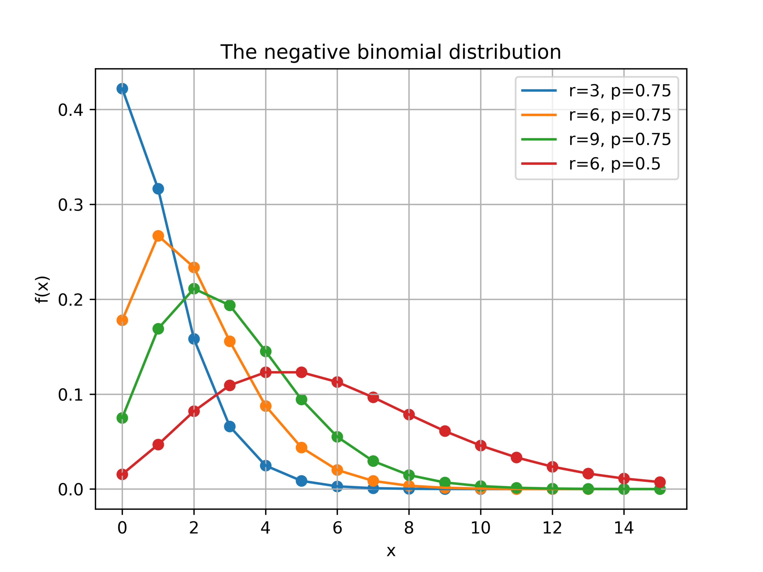
    The negative binomial distribution describes the number of times a coin lands on tails before a certain number of heads are recorded. The distribution depends on two parameters \(p\) and \(r\). The parameter \(p\) is the probability that the coin lands on heads and \(r\) is the number of heads. If \(X\) has the negative binomial distribution, then \(X = x\) means in the first \(x+r-1\) tosses of the coin, there were \(r-1\) heads and that toss number \(x+r\) was a head. This means that the probability that \(X=x\) is given by

    \(\displaystyle{f(x) = \binom{x+r-1}{r-1}p^{r}\left(1-p\right)^x}\)

    Here is a plot of the function \(f(x)\) for different values of \(r\) and \(p\).

    Poisson approximations

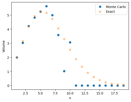
    When the parameter \(r\) is large and \(p\) is close to one, the negative binomial distribution can be approximated by a Poisson distribution. More formally, suppose that \(r(1-p)=\lambda\) for some positive real number \(\lambda\). If \(r\) is large then, the negative binomial random variable with parameters \(p\) and \(r\), converges to a Poisson random variable with parameter \(\lambda\). This is illustrated in the picture below where three negative binomial distributions with \(r(1-p)=5\) approach the Poisson distribution with \(\lambda =5\).

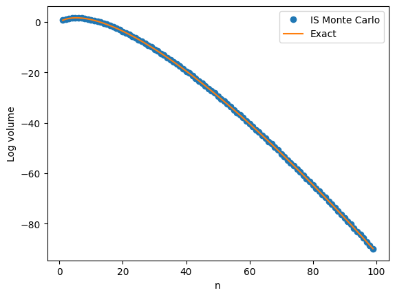
    Total variation distance is a common way to measure the distance between two discrete probability distributions. The log-log plot below shows that the error from the Poisson approximation is on the order of \(1/r\) and that the error is bigger if the limiting value of \(r(1-p)\) is larger.

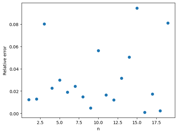
    It turns out that is is possible to get a more accurate approximation by using a different Poisson distribution. In the first approximation, we used a Poisson random variable with mean \(\lambda = r(1-p)\). However, the mean of the negative binomial distribution is \(r(1-p)/p\). This suggests that we can get a better approximation by setting \(\lambda = r(1-p)/p\).

    The change from \(\lambda = r(1-p)\) to \(\lambda = r(1-p)/p\) is a small because \(p \approx 1\). However, this small change gives a much better approximation, especially for larger values of \(r(1-p)\). The below plot shows that both approximations have errors on the order of \(1/r\), but the constant for the second approximation is much better.

    Second order accurate approximation

    It is possible to further improve the Poisson approximation by using a Gram–Charlier expansion. A Gram–Charlier approximation for the Poisson distribution is given in this paper.1 The approximation is

    \(\displaystyle{f_{GC}(x) = P_\lambda(x) – \frac{1}{2}(1-p)\left((x-\lambda)P_\lambda(x)-(x-1-\lambda)P_\lambda(x-1)\right)},\)

    where \(\lambda = \frac{k(1-p)}{p}\) as in the second Poisson approximation and \(P_\lambda(x)\) is the Poisson pmf evaluated at \(x\).

    The Gram–Charlier expansion is considerably more accurate than either Poisson approximation. The errors are on the order of \(1/r^2\). This higher accuracy means that the error curves for the Gram–Charlier expansion has a steeper slope.

    1. The approximation is given in equation (4) of the paper and is stated in terms of the CDF instead of the PMF. The equation also contains a small typo, it should say \(\frac{1}{2}q\) instead of \(\frac{1}{2}p\). ↩︎
  • Understanding the Ratio of Uniforms Distribution

    The ratio of uniforms distribution is a useful distribution for rejection sampling. It gives a simple and fast way to sample from discrete distributions like the hypergeometric distribution1. To use the ratio of uniforms distribution in rejection sampling, we need to know the distributions density. This post summarizes some properties of the ratio of uniforms distribution and computes its density.

    The ratio of uniforms distribution is the distribution of the ratio of two independent uniform random variables. Specifically, suppose \(U \in [-1,1]\) and \(V \in [0,1]\) are independent and uniformly distributed. Then \(R = U/V\) has the ratio of uniforms distribution. The plot below shows a histogram based on 10,000 samples from the ratio of uniforms distribution2.

    The histogram has a flat section in the middle and then curves down on either side. This distinctive shape is called a “table mountain”. The density of \(R\) also has a table mountain shape.

    And here is the density plotted on top of the histogram.

    A formula for the density of \(R\) is

    \(\displaystyle{h(R) = \begin{cases} \frac{1}{4} & \text{if } -1 \le R \le 1, \\\frac{1}{4R^2} & \text{if } R < -1 \text{ or } R > 1.\end{cases}}\)

    The first case in the definition of \(h\) corresponds to the flat part of the table mountain. The second case corresponds to the sloping curves. The rest of this post use geometry to derive the above formula for \(h(R)\).

    Calculating the density

    The point \((U,V)\) is uniformly distributed in the box \(B=[-1,1] \times [0,1]\). The image below shows an example of a point \((U,V)\) inside the box \(B\).

    We can compute the ratio \(R = U/V\) geometrically. First we draw a straight line that starts at \((0,0)\) and goes through \((U,V)\). This line will hit the horizontal line \(y=1\). The \(x\) coordinate at this point is exactly \(R=U/V\).

    In the above picture, all of the points on the dashed line map to the same value of \(R\). We can compute the density of \(R\) by computing an area. The probability that \(R\) is in a small interval \([R,R+dR]\) is

    \(\displaystyle{\frac{\text{Area}(\{(u,v) \in B : u/v \in [R, R+dR]\})}{\text{Area}(B)} = \frac{1}{2}\text{Area}(\{(u,v) \in B : u/v \in [R, R+dR]\}).}\)

    If we can compute the above area, then we will know the density of \(R\) because by definition

    \(\displaystyle{h(R) = \lim_{dR \to 0} \frac{1}{2dR}\text{Area}(\{(u,v) \in B : u/v \in [R, R+dR]\})}.\)

    We will first work on the case when \(R\) is between \(-1\) and \(1\). In this case, the set \(\{(u,v) \in B : u/v \in [R, R+dR]\}\) is a triangle. This triangle is drawn in blue below.

    The horizontal edge of this triangle has length \(dR\). The perpendicular height of the triangle from the horizontal edge is \(1\). This means that

    \( \displaystyle{\text{Area}(\{(u,v) \in B : u/v \in [R, R+dR]\}) =\frac{1}{2}\times dR \times 1=\frac{dR}{2}}.\)

    And so, when \(R \in [-1,1]\) we have

    \(\displaystyle{h(R) = \lim_{dR\to 0} \frac{1}{2dR}\times \frac{dR}{2}=\frac{1}{4}}.\)

    Now let’s work on the case when \(R\) is bigger than \(1\) or less than \(-1\). In this case, the set \(\{(u,v) \in B : u/v \in [R, R+dR]\}\) is again triangle. But now the triangle has a vertical edge and is much skinnier. Below the triangle is drawn in red. Note that only points inside the box \(B\) are coloured in.

    The vertical edge of the triangle has length \(\frac{1}{R} – \frac{1}{R+dR}= \frac{dR}{R(R+dR)}\). The perpendicular height of the triangle from the vertical edge is \(1\). Putting this together

    \( \displaystyle{\text{Area}(\{(u,v) \in B : u/v \in [R, R+dR]\}) =\frac{1}{2}\times \frac{dR}{R(R+dR)} \times 1=\frac{dR}{2R(R+dR)}}.\)

    And so

    \(\displaystyle{h(R) = \lim_{dR \to 0} \frac{1}{2dR} \times \frac{dR}{2 R(R+dR)} = \frac{1}{4R^2}}.\)

    And so putting everything together

    \(\displaystyle{h(R) = \begin{cases} \frac{1}{4} & \text{if } -1 \le R \le 1, \\\frac{1}{4R^2} & \text{if } R < -1 \text{ or } R > 1.\end{cases}}\)

    Footnotes and references

    1. https://ieeexplore.ieee.org/document/718718 ↩︎
    2. For visual purposes, I restricted the sample to values of \(R\) between \(-8\) and \(8\). This is because the ratio of uniform distribution has heavy tails. This meant that there were some very large values of \(R\) that made the plot hard to see. ↩︎
  • The sample size required for importance sampling

    My last post was about using importance sampling to estimate the volume of high-dimensional ball. The two figures below compare plain Monte Carlo to using importance sampling with a Gaussian proposal. Both plots use \(M=1,000\) samples to estimate \(v_n\), the volume of an \(n\)-dimensional ball

    A friend of mine pointed out that the relative error does not seem to increase with the dimension \(n\). He thought it was too good to be true. It turns out he was right and the relative error does increase with dimension but it increases very slowly. To estimate \(v_n\) the number of samples needs to grow on the order of \(\sqrt{n}\).

    To prove this, we will use the paper The sample size required for importance sampling by Chatterjee and Diaconis [1]. This paper shows that the sample size for importance sampling is determined by the Kullback-Liebler divergence. The relevant result from their paper is Theorem 1.3. This theorem is about the relative error in using importance sampling to estimate a probability.

    In our setting the proposal distribution is \(Q=\mathcal{N}(0,\frac{1}{n}I_n)\). That is the distribution \(Q\) is an \(n\)-dimensional Gaussian vector with mean \(0\) and covariance \(\frac{1}{n}I_n\). The conditional target distribution is \(P\) the uniform distribution on the \(n\) dimensional ball. Theorem 1.3 in [1] tells us how many samples are needed to estimate \(v_n\). Informally, the required sample size is \(M = O(\exp(D(P \Vert Q)))\). Here \(D(P\Vert Q)\) is the Kullback-Liebler divergence between \(P\) and \(Q\).

    To use this theorem we need to compute \(D(P \Vert Q)\). Kullback-Liebler divergence is defined as integral. Specifically

    \(\displaystyle{D(P\Vert Q) = \int_{\mathbb{R}^n} \log\frac{P(x)}{Q(x)}P(x)dx}\)

    Computing the high-dimensional integral above looks challenging. Fortunately, it can reduced to a one-dimensional integral. This is because both the distributions \(P\) and \(Q\) are rotationally symmetric. To use this, define \(P_r,Q_r\) to be the distribution of the norm squared under \(P\) and \(Q\). That is if \(X \sim P\), then \(\Vert X \Vert_2^2 \sim P_R\) and likewise for \(Q_R\). By the rotational symmetry of \(P\) and \(Q\) we have

    \(D(P\Vert Q) = D(P_R \Vert Q_R).\)

    We can work out both \(P_R\) and \(Q_R\). The distribution \(P\) is the uniform distribution on the \(n\)-dimensional ball. And so for \(X \sim P\) and any \(r \in [0,1]\)

    \(\mathbb{P}(\Vert X \Vert_2^2 \le r) = \frac{v_n r^n}{v_n} = r^n.\)

    Which implies that \(P_R\) has density \(P_R(r)=nr^{n-1}\). This means that \(P_R\) is a Beta distribution with parameters \(\alpha = n, \beta = 1\). The distribution \(Q\) is a multivariate Gaussian distribution with mean \(0\) and variance \(\frac{1}{n}I_n\). This means that if \(X \sim Q\), then \(\Vert X \Vert_2^2 = \sum_{i=1}^n X_i^2\) is a scaled chi-squared variable. The shape parameter of \(Q_R\) is \(n\) and scale parameter is \(1/n\). The density for \(Q_R\) is therefor

    \(Q_R(r) = \frac{n^{n/2}}{2^{n/2}\Gamma(n/2)}r^{n/2-1}e^{-nx/2}\)

    The Kullback-Leibler divergence between \(P\) and \(Q\) is therefor

    \(\displaystyle{D(P\Vert Q)=D(P_R\Vert Q_R) = \int_0^1 \log \frac{P_R(r)}{Q_R(r)} P_R(r)dr}\)

    Getting Mathematica to do the above integral gives

    \(D(P \Vert Q) = -\frac{1+2n}{2+2n} + \frac{n}{2}\log(2 e) – (1-\frac{n}{2})\log n + \log \Gamma(\frac{n}{2}).\)

    Using the approximation \(\log \Gamma(z) \approx (z-\frac{1}{2})\log(z)-z+O(1)\) we get that for large \(n\)

    \(D(P \Vert Q) = \frac{1}{2}\log n + O(1)\).

    And so the required number of samples is \(O(\exp(D(P \Vert Q)) = O(\sqrt{n}).\)

    [1] Chatterjee, Sourav, and Persi Diaconis. “THE SAMPLE SIZE REQUIRED IN IMPORTANCE SAMPLING.” The Annals of Applied Probability 28, no. 2 (2018): 1099–1135. https://www.jstor.org/stable/26542331. (Public preprint here https://arxiv.org/abs/1511.01437)

  • Monte Carlo integration in high dimensions

    Monte Carlo integration

    John Cook recently wrote a cautionary blog post about using Monte Carlo to estimate the volume of a high-dimensional ball. He points out that if \(\mathbf{X}=(X_1,\ldots,X_n)\) are independent and uniformly distributed on the interval \([-1,1]\) then

    \(\displaystyle{\mathbb{P}(X_1^2 + X_2^2 + \cdots + X_n^2 \le 1) = \frac{v_n}{2^n}},\)

    where \(v_n\) is the volume of an \(n\)-dimensional ball with radius one. This observation means that we can use Monte Carlo to estimate \(v_n\).

    To do this we repeatedly sample vectors \(\mathbf{X}_m = (X_{m,1},\ldots,X_{m,n})\) with \(X_{m,i}\) uniform on \([-1,1]\) and \(m\) ranging from \(1\) to \(M\). Next, we count the proportion of vectors \(\mathbf{X}_m\) with \(X_{1,m}^2 + \cdots + X_{n,m}^2 \le 1\). Specifically, if \(Z_m\) is equal to one when \(X_{1,m}^2 + \cdots + X_{n,m}^2 \le 1\) and equal to zero otherwise, then by the law of large numbers

    \(\displaystyle{\frac{1}{M}\sum_{m=1}^M Z_m \approx \frac{v_n}{2^n}}\)

    Which implies

    \(v_n \approx 2^n \frac{1}{M}\sum_{m=1}^M Z_m\)

    This method of approximating a volume or integral by sampling and counting is called Monte Carlo integration and is a powerful general tool in scientific computing.

    The problem with Monte Carlo integration

    As pointed out by John, Monte Carlo integration does not work very well in this example. The plot below shows a large difference between the true value of \(v_n\) with \(n\) ranging from \(1\) to \(20\) and the Monte Carlo approximation with \(M = 1,000\).

    The problem is that \(v_n\) is very small and the probability \(v_n/2^n\) is even smaller! For example when \(n = 10\), \(v_n/2^n \approx 0.0025\). This means that in our one thousand samples we only expect two or three occurrences of the event \(X_{m,1}^2 + \cdots + X_{m,n}^2 \le 1\). As a result our estimate has a high variance.

    The results get even worse as \(n\) increases. The probability \(v_n/2^n\) does to zero faster than exponentially. Even with a large value of \(M\), our estimate will be zero. Since \(v_n \neq 0\), the relative error in the approximation is 100%.

    Importance sampling

    Monte Carlo can still be used to approximate \(v_n\). Instead of using plain Monte Carlo, we can use a variance reduction technique called importance sampling (IS). Instead of sampling the points \(X_{m,1},\ldots, X_{m,n}\) from the uniform distribution on \([-1,1]\), we can instead sample the from some other distribution called a proposal distribution. The proposal distribution should be chosen so that that the event \(X_{m,1}^2 +\cdots +X_{m,n}^2 \le 1\) becomes more likely.

    In importance sampling, we need to correct for the fact that we are using a new distribution instead of the uniform distribution. Instead of the counting the number of times \(X_{m,1}^2+\cdots+X_{m,n}^2 \le 1\) , we give weights to each of samples and then add up the weights.

    If \(p\) is the density of the uniform distribution on \([-1,1]\) (the target distribution) and \(q\) is the density of the proposal distribution, then the IS Monte Carlo estimate of \(v_n\) is

    \(\displaystyle{\frac{1}{M}\sum_{m=1}^M Z_m \prod_{i=1}^n \frac{p(X_{m,i})}{q(X_{m,i})}},\)

    where as before \(Z_m\) is one if \(X_{m,1}^2+\cdots +X_{m,n}^2 \le 1\) and \(Z_m\) is zero otherwise. As long as \(q(x)=0\) implies \(p(x)=0\), the IS Monte Carlo estimate will be an unbiased estimate of \(v_n\). More importantly, a good choice of the proposal distribution \(q\) can drastically reduce the variance of the IS estimate compared to the plain Monte Carlo estimate.

    In this example, a good choice of proposal distribution is the normal distribution with mean \(0\) and variance \(1/n\). Under this proposal distribution, the expected value of \(X_{m,1}^2 +\cdots+ X_{m,n}^2\) is one and so the event \(X_{m,1}^2 + \cdots + X_{m,n}^2 \le 1\) is much more likely.

    Here are the IS Monte Carlo estimates with again \(M = 1,000\) and \(n\) ranging from \(1\) to \(20\). The results speak for themselves.

    The relative error is typically less than 10%. A big improvement over the 100% relative error of plain Monte Carlo.

    The next plot shows a close agreement between \(v_n\) and the IS Monte Carlo approximation on the log scale with \(n\) going all the way up to \(100\).

    Notes

    1. There are exact formulas for \(v_n\) (available on Wikipedia). I used these to compare the approximations and compute relative errors. There are related problems where no formulas exist and Monte Carlo integration is one of the only ways to get an approximate answer.
    2. The post by John Cook also talks about why the central limit theorem can’t be used to approximate \(v_n\). I initially thought a technique called large deviations could be used to approximate \(v_n\) but again this does not directly apply. I was happy to discover that importance sampling worked so well!

    More sampling posts

  • Solving a system of equations vs inverting a matrix

    I used to have trouble understanding why inverting an \(n \times n\) matrix required the same order of operations as solving an \(n \times n\) system of linear equations. Specifically, if \(A\) is an \(n\times n\) invertible matrix and \(b\) is a length \(n\) vector, then computing \(A^{-1}\) and solving the equation \(Ax = b\) can both be done in \(O(n^3)\) floating point operations (flops). This surprised me because naively computing the columns of \(A^{-1}\) requires solving the \(n\) systems of equations

    \(Ax = e_1, Ax=e_2,\ldots, Ax = e_n,\)

    where \(e_1,e_2,\ldots, e_n\) are the standard basis vectors. I thought this would mean that calculating \(A^{-1}\) would require roughly \(n\) times as many flops as solving a single system of equations. It was only in a convex optimization lecture that I realized what was going on.

    To solve a single system of equations \(Ax = b\), we first compute a factorization of \(A\) such as the LU factorization. Computing this factorization takes \(O(n^3)\) flops but once we have it, we can use it solve any new system with \(O(n^2)\) flops. Now to solve \(Ax=e_1,Ax=e_2,\ldots,Ax=e_n\), we can simply factor \(A\) once and the perform \(n\) solves using the factorization each of which requires an addition \(O(n^2)\) flops. The total flop count is then \(O(n^3)+nO(n^2)=O(n^3)\). Inverting the matrix requires the same order of flops as a single solve!

    Of course, as John D Cook points out: you shouldn’t ever invert a matrix. Even if inverting and solving take the same order of flops, inverting is still more computational expensive and requires more memory.

    Related posts