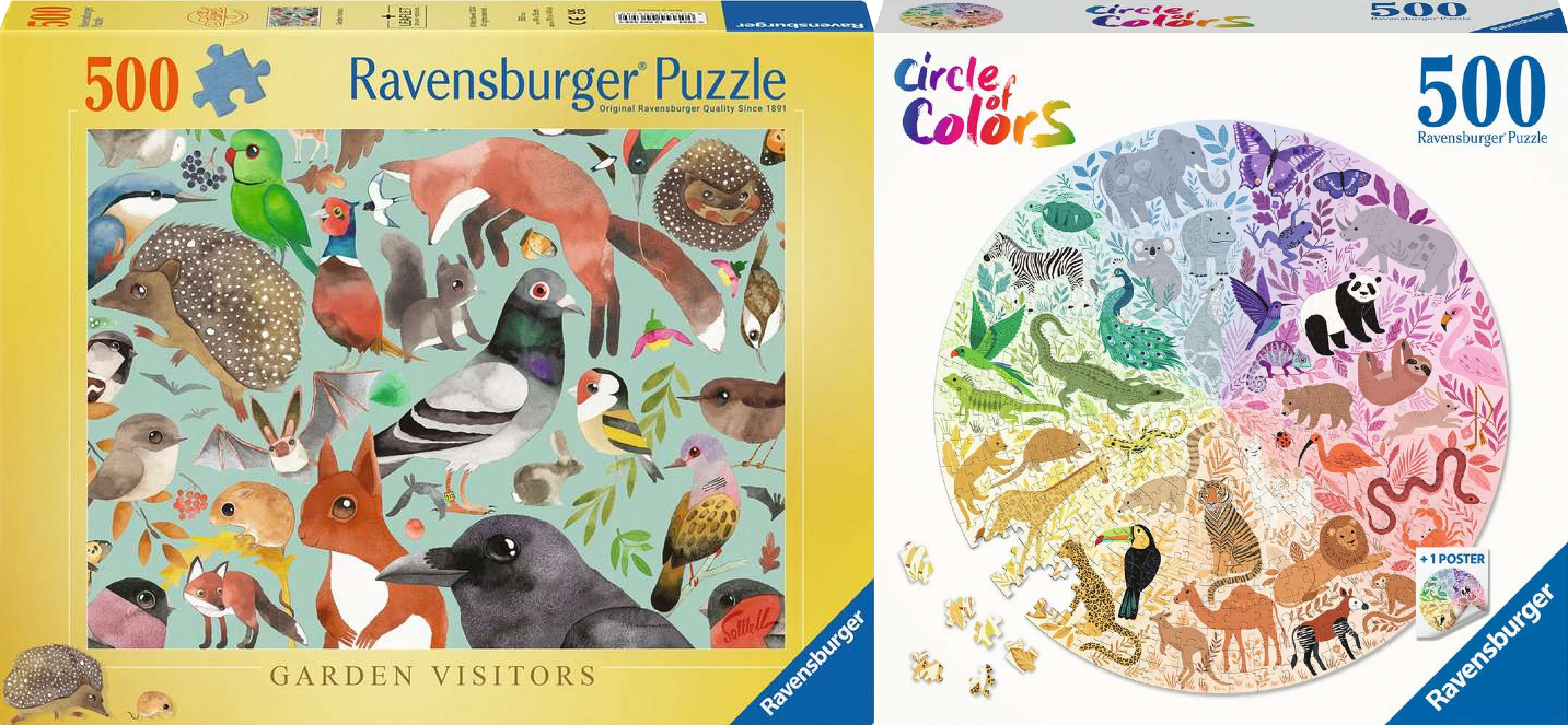
The 2025 World Jigsaw Puzzle Championship recently took place in Spain. In the individual heats, competitors had to choose their puzzle. Each competitor could either complete a 500-piece rectangular puzzle or a 500-piece circular puzzle. For example, in Round F, puzzlers could choose one of the following two puzzles:
There are many things to consider when picking a puzzle. First, the puzzles had already been released. This meant a puzzler could get an advantage by choosing to do a puzzle they had already completed. The image on the puzzle is also important, as is the puzzle’s style. In the example above, most puzzlers picked the circular puzzle because it had a clear colour gradient and distinct sections.
The commentators mentioned that puzzlers might also consider the number of edge pieces. The circular puzzles have fewer edge pieces than the rectangular puzzles. This could make the rectangular puzzle easier because some puzzlers like to do the edge first and then build inwards.
The difference in edge pieces isn’t a coincidence. Circular puzzles have fewer edge pieces than any other 500-piece puzzle. This fact is a consequence of a piece of mathematics called the isoperimetric inequality.
The isopermetric inequality
The isoperimetric inequality is a statement about 2D shapes. The word ‘isoperimetric’ literally translates to ‘having the same perimeter.’ The isoperimetric inequality says that if a shape has the same perimeter as a particular circle, then the circle has a larger (or equal) area. For example, the square and circle below have the same perimeter but the circle has a larger area:
The isoperimetric inequality can also be flipped around to give a statement about shapes with the same area. This ‘having the same area’ inequality states that if a shape has the same area as a circle, then the circle has a smaller (or equal) perimeter. For example, the square and circle below have the same area but the circle has a smaller perimeter:
The ‘having the same area’ inequality applies to the jigsaw puzzles above. In a jigsaw puzzle, the area is proportional to the number of pieces and the perimeter is proportional to the number of edge pieces (assuming the pieces are all roughly the same size and shape). This means that if one puzzle has the same number of pieces as a circular puzzle (for example 500), then the circular puzzle will have fewer edge pieces! This is exactly what the commentator said about the puzzles in the competition!
I don’t think many of the puzzlers thought about the isopermetric inequality when picking their puzzles. But if you ever do a circular puzzle, remember that you’re doing a puzzle with as few edge pieces as possible!
Growing up, my siblings and I would read a lot of Bill Watterson’s Calvin and Hobbes. I have fond memories of spending hours reading and re-reading our grandparents collection during the school holidays. The comic strip is witty, heartwarming and beautifully drawn.
Seeing Calvin take this test took me back to those school holidays. I remember grabbing paper and a pencil to work out the answer (I also remember getting teased by those previously mentioned siblings). Reading the strip years later, I realized there’s a neat way to work out the answer without having to write much down. Here’s the question again,
Jack and Joe leave their homes at the same time and drive toward each other. Jack drives at 60 mph, while Joe drives at 30 mph. They pass each other in 10 minutes.
How far apart were Jack and Joe when they started?
It can be hard to think about Jack and Joe traveling at different speeds. But we can simplify the problem by thinking from Joe’s perspective or frame of reference. From Joe’s frame of reference, he is staying perfectly still but Jack is zooming towards him at \(30+60=90\) mph. Jack reaches Joe in 10 minutes which is one sixth of an hour. This means that the initial distance between them must have been \(90 \times 1/6 = 15\) miles.
It’s not as creative as Calvin’s private eye approach but at least Susie and I got the same answer.
A few months ago, I had the pleasure of reading Eugenia Cheng‘s book How to Bake Pi. Each chapter starts with a recipe which Cheng links to the mathematical concepts contained in the chapter. The book is full of interesting connections between mathematics and the rest of the world.
One of my favourite ideas in the book is something Cheng writes about equations and the humble equals sign: \(=\). She explains that when an equation says two things are equal we very rarely mean that they are exactly the same thing. What we really mean is that the two things are the same in some ways even though they may be different in others.
One example that Cheng gives is the equation \(a + b = b+a\). This is such a familiar statement that you might really think that \(a+b\) and \(b+a\) are the same thing. Indeed, if \(a\) and \(b\) are any numbers, then the number you get when you calculate \(a + b\) is the same as the number you get when you calculate \(b + a\). But calculating \(a+b\) could be very different from calculating \(b+a\). A young child might calculate \(a+b\) by starting with \(a\) and then counting one-by-one from \(a\) to \(a + b\). If \(a\) is \(1\) and \(b\) is \(20\), then calculating \(a + b\) requires counting from \(1\) to \(21\) but calculating \(b+a\) simply amounts to counting from \(20\) to \(21\). The first process takes way longer than the second and the child might disagree that \(1 + 20\) is the same as \(20 + 1\).
In How to Bake Pi, Cheng explains that a crucial idea behind equality is context. When someone says that two things are equal we really mean that they are equal in the context we care about. Cheng talks about how context is crucial through-out mathematics and introduces a little bit of category theory as a tool for moving between different contexts. I think that this idea of context is really illuminating and I wanted to share some examples where “\(=\)” doesn’t mean “exactly the same as”.
The Sherman-Morrison formula
The Sherman-Morrison formula is a result from linear algebra that says for any invertible matrix \(A \in \mathbb{R}^{n\times n}\) and any pair of vectors \(u,v \in \mathbb{R}^n\), if \(v^TA^{-1}u \neq -1\), then \(A + uv^T\) is invertible and
You can take any natural number \(n\), any matrix \(A\) of size \(n\) by \(n\), and any length \(n\)-vectors \(u\) and \(v\) that satisfy the above condition.
If you take all those things and carry out all the matrix multiplications, additions and inversions on the left and all the matrix multiplications, additions and inversions on the right, then you will end up with exactly the same matrix in both cases.
But depending on the context, the equation on one side of “\(=\)” may be much easier than the other. Although the right hand side looks a lot more complicated, it is much easier to compute in one important context. This context is when we have already calculated the matrix \(A^{-1}\) and now want the inverse of \(A + uv^T\). The left hand side naively computes \(A + uv^T\) which takes \(O(n^3)\) computations since we have to invert a \(n \times n\) matrix. On the right hand side, we only need to compute a small number of matrix-vector products and then add two matrices together. This bring the computational cost down to \(O(n^2)\).
These cost saving measures come up a lot when studying linear regression. The Sherman-Morrison formula can be used to update regression coefficients when a new data point is added. Similarly, the Sherman-Morrison formula can be used to quickly calculate the fitted values in leave-one-out cross validation.
log-sum-exp
This second example also has connections to statistics. In a mixture model, we assume that each data point \(Y\) comes from a distribution of the form:
where \(\pi \) is a vector and \(\pi_k\) is equal to the probability that \(Y\) came from class \(k\). The parameters \(\theta_k \in\mathbb{R}^p\) are the parameters for the \(k^{th}\) group.The log-likelihood is thus,
where \(\eta_{k} = \log(\pi_k p(y| \theta_k))\). We can see that the log-likelihood is of the form log-sum-exp. Calculating a log-sum-exp can cause issues with numerical stability. For instance if \(K = 3\) and \(\eta_k = 1000\), for all \(k=1,2,3\), then the final answer is simply \(\log(3)+1000\). However, as soon as we try to calculate \(\exp(1000)\) on a computer, we’ll be in trouble.
The solution is to use the following equality, for any \(\beta \in \mathbb{R}\),
Proving the above identity is a nice exercise in the laws of logarithm’s and exponential’s, but with a clever choice of \(\beta\) we can more safely compute the log-sum-exp expression. For instance, in the documentation for pytorch’s implementation of logsumexp() they take \(\beta\) to be the maximum of \(\eta_k\). This (hopefully) makes each of the terms \(\beta – \eta_k\) a reasonable size and avoids any numerical issues.
Again, the left and right hand sides of the above equation might be the same number, but in the context of having to use computers with limited precision, they represent very different calculations.
Beyond How to Bake Pi
Eugenia Cheng has recently published a new book called The Joy of Abstraction. I’m just over half way through and it’s been a really engaging and interesting introduction to category theory. I’m looking forward to reading the rest of it and getting more insight from Eugenia Cheng’s great mathematical writing.
Next week I’ll be starting the second year of my statistics PhD. I’ve learnt a lot from taking the first year classes and studying for the qualifying exams. Some of what I’ve learnt has given me a new perspective on some of my old blog posts. Here are three things that I’ve written about before and I now understand better.
1. The Pi-Lambda Theorem
An early post on this blog was titled “A minimal counterexample in probability theory“. The post was about a theorem from the probability course offered at the Australian National University. The theorem states that if two probability measures agree on a collection of subsets and the collection is closed under finite intersections, then the two probability measures agree on the \(\sigma\)-algebra generated by the collection. In my post I give an example which shows that you need the collection to be closed under finite intersections. I also show that you need to have at least four points in the space to find such an example.
What I didn’t know then is that the above theorem is really a corollary of Dykin’s \(\pi – \lambda\) theorem. This theorem was proved in my first graduate probability course which was taught by Persi Diaconis. Professor Diaconis kept a running tally of how many times we used the \(\pi – \lambda\) theorem in his course and we got up to at least 10. (For more appearances by Professor Diaconis on this blog see here, here and here).
If I were to write the above post again, I would talk about the \(\pi – \lambda\) theorem and rename the post “The smallest \(\lambda\)-system”. The example given in my post is really about needing at least four points to find a \(\lambda\)-system that is not a \(\sigma\)-algebra.
2. Mallow’s Cp statistic
The very first blog post I wrote was called “Complexity Penalties in Statistical Learning“. I wasn’t sure if I would write a second and so I didn’t set up a WordPress account. I instead put the post on the website LessWrong. I no longer associate myself with the rationality community but posting to LessWrong was straight forward and helped me reach more people.
The post was inspired in two ways by the 2019 AMSI summer school. First, the content is from the statistical learning course I took at the summer school. Second, at the career fair many employers advised us to work on our writing skills. I don’t know if would have started blogging if not for the AMSI Summer School.
I didn’t know it at the time but the blog post is really about Mallow’s Cp statistic. Mallow’s Cp statistic is an estimate of the test error of a regression model fit using ordinary least squares. The Mallow’s Cp is equal to the training error plus a “complexity penalty” which takes into account the number of parameters. In the blog post I talk about model complexity and over-fitting. I also write down and explain Mallow’s Cp in the special case of polynomial regression.
In the summer school course I took, I don’t remember the name Mallow’s Cp being used but I thought it was a great idea and enjoyed writing about it. The next time encountered Mallow’s Cp was in the linear models course I took last fall. I was delighted to see it again and learn how it fit into a bigger picture. More recently, I read Brad Efron’s paper “How Biased is the Apparent Error Rate of a Prediction Rule?“. The paper introduces the idea of “effective degrees of freedom” and expands on the ideas behind the Cp statistic.
Incidentally, enrolment is now open for the 2023 AMSI Summer School! This summer it will be hosted at the University of Melbourne. I encourage any Australia mathematics or statistics students reading this to take a look and apply. I really enjoyed going in both 2019 and 2020. (Also if you click on the above link you can try to spot me in the group photo of everyone wearing read shirts!)
3. Finitely additive probability measures
In “Finitely additive measures” I talk about how hard it is to define a finitely additive measure on the set of natural numbers that is not countably additive. In particular, I talked about needing to use the Hahn — Banach extension theorem to extend the natural density from the collection of sets with density to the collection of all subsets of the natural numbers.
There were a number of homework problems in my first graduate probability course that relate to this post. We proved that the sets with density are not closed under finite unions and we showed that the square free numbers have density \(6/\pi^2\).
We also proved that any finite measure defined on an algebra of subsets can be extend to the collection of all subsets. This proof used Zorn’s lemma and the resulting measure is far from unique. The use of Zorn’s lemma relates to the main idea in my blog, that defining an additive probability measure is in some sense non-constructive.
Other posts
Going forward, I hope to continue publishing at least one new post every month. I look forward to one day writing another post like this when I can look back and reflect on how much I have learnt.
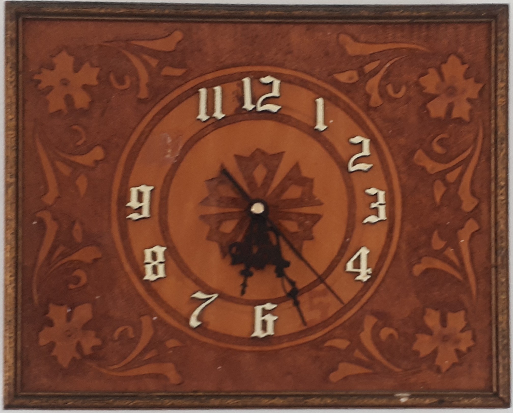
Recently, my partner and I installed a clock in our home. The clock previously belonged to my grandparents and we have owned it for a while. We hadn’t put it up earlier because the original clock movement ticked and the sound would disrupt our small studio apartment. After much procrastinating, I bought a new clock movement, replaced the old one and proudly hung up our clock.
Our new clock. We still need to reattach the 5 and 10 which fell off when we moved.
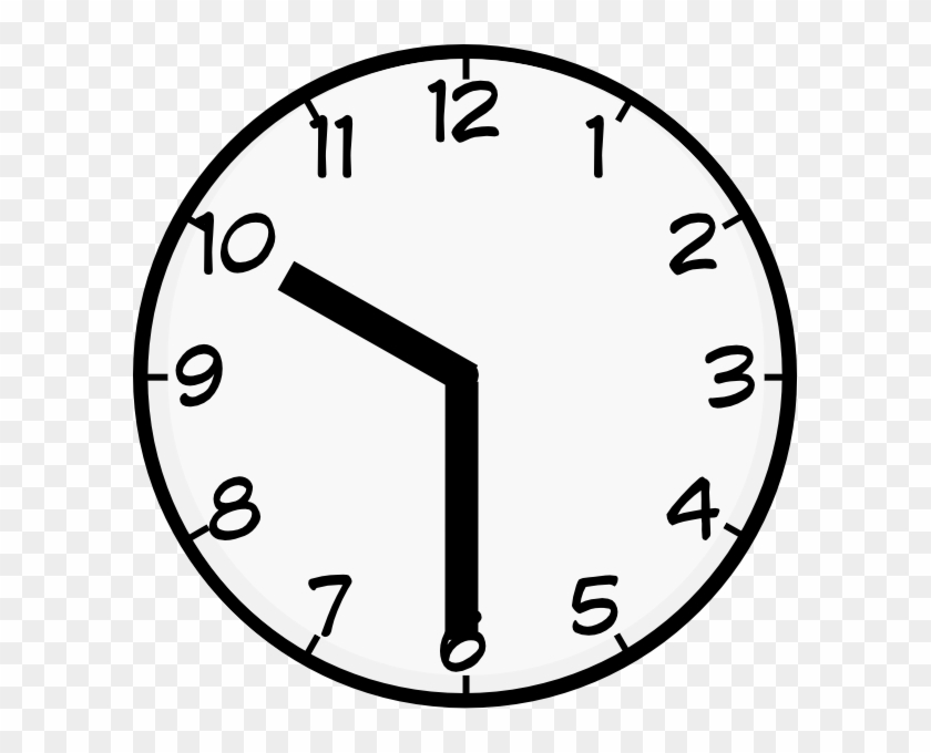
When I first put on the clock hands I made the mistake of not putting them both on at exactly 12 o’clock. This meant that the minute and hour hands were not synchronised. The hands were in an impossible position. At times, the minute hand was at 12 and the hour hand was between 3 and 4. It took some time for me to register my mistake as at some times of the day it can be hard to tell that the hands are out of sync (how often do you look at a clock at 12:00 exactly?). Fortunately, I did notice the mistake and we have a correct clock. Now I can’t help noticing when others make the same mistake such as in this piece of clip art.
After fixing the clock, I was still thinking about how only some clock hand positions correspond to actual times. This led me to think “a clock is a one-dimensional subgroup of the torus”. Let me explain why.
The torus
The minute and hour hands on a clock can be thought of as two points on two different circles. For instance, if the time is 9:30, then the minute hand corresponds to a point at the very bottom of the circle and the hour hand corresponds to a point 15 degrees clockwise of the leftmost point of the circle. As a clock goes through a 12 hour cycle the minute-hand-point goes around the circle 12 times and the hour-hand-point goes around the circle once. This is shown below.
The blue point goes around its blue circle in time with the minute hand on the clock in the middle. The red point goes around its red circle in time with the hour hand.
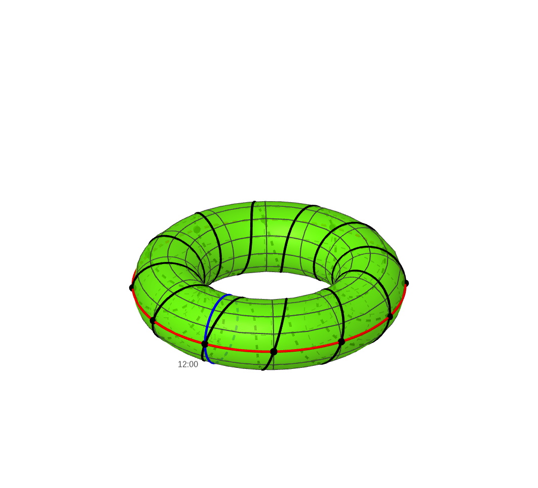
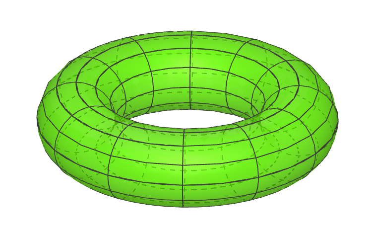
If you take the collection of all pairs of points on a circle you get what mathematicians call a torus. The torus is a geometric shape that looks like the surface of a donut. The torus is defined as the Cartesian product of two circles. That is, a single point on the torus corresponds to two points on two different circles. A torus is plotted below.
The green surface above is a torus. The black lines aren’t a part of the torus, they are just there to help the visualisation.
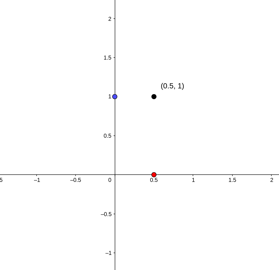
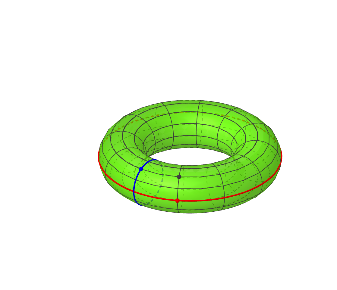
To understand the torus, it’s helpful to consider a more familiar example, the 2-dimensional plane. If we have points \(x\) and \(y\) on two different lines, then we can produce the point \((x,y)\) in the two dimensional plane. Likewise, if we have a point \(p\) and a point \(q\) on two different circles, then we can produce a point \((p,q)\) on the torus. Both of these concepts are illustrated below. I have added two circles to the torus which are analogous to the x and y axes of the plane. The blue and red points on the blue and red circle produce the black point on the torus.
Mapping the clock to the torus
The points on the torus are in one-to-one correspondence with possible arrangements of the two clock hands. However, as I learnt putting up our clock, not all arrangements of clock hands correspond to an actual time. This means that only some points on the torus correspond to an actual time but how can we identify these points?
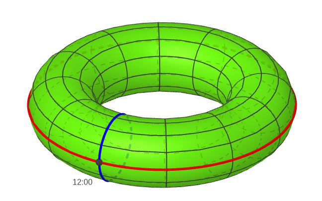
Keeping with our previous convention, let’s use the blue circle to represent the position of the minute hand and the red circle to represent the position of the hour hand. This means that the point where the two circles meet corresponds to 12 o’clock.
The point where the two circles meet corresponds to both hands pointing to 12, that is, 12 o’clock.
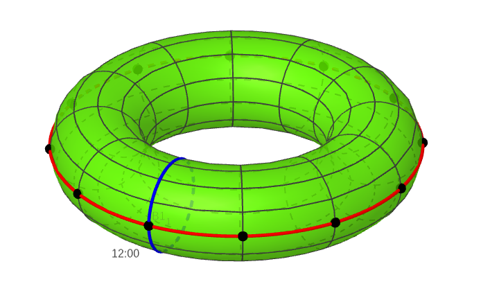
There are eleven other points on the red line that correspond to the other times when the minute hand is at 12. That is, there’s a point for 1 o’clock, 2 o’clock, 3 o’clock and so on. Once we add in those points, our torus looks like this:
Each black dot corresponds to when the minute hand is at 12. That is, the dots represent 12 o’clock, 1 o’clock, 2 o’clock and so on.
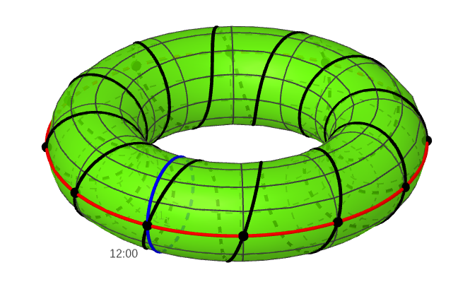
Finally, we have to join these points together. We know that when the hour hand moves from 12 to 1, the minute hand does one full rotation. This means that we have to join the black points by making one full rotation in the direction of the blue circle. The result is the black curve below that snakes around the torus.
Points on the black curve correspond to actual times on the clock.
The picture above should explain most of this blog’s title – “a clock is a one-dimensional subgroup of the torus”. We now know what the torus is and why certain points on the torus correspond to positions of the hands on a clock. We can see that these “clock points” correspond to a line that snakes around the torus. While the torus is a surface and hence two dimensional, the line is one-dimensional. The last missing part is the word “subgroup”. I won’t go into the details here but the torus has some extra structure that makes it something called a group. Our map from the clock to the torus interacts nicely with this structure and this makes the black line a “subgroup”.
Another perspective
While the above pictures of the torus are pretty, they can be a bit hard to understand and hard to draw. Mathematicians have another perspective of the torus that is often easier to work with. Imagine that you have a square sheet of rubber. If you rolled up the rubber and joined a pair of opposite sides, you would get a rubber tube. If you then bent the tube to join the opposite sides again, you would get a torus! The gif bellow illustrates this idea
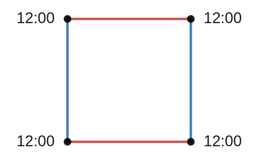
This means that we can simply view the torus as a square. We just have to remember that the opposite sides of the squares have been glued together. So like a game of snake on a phone, if you leave the top of the square, you come out at the same place on the bottom of the square. If we use this idea to redraw our torus it now looks like this:
A drawing of a flat torus. To make a donut shaped torus, the two red lines and then the two blue lines have to be glued together. As before, the blue line corresponds to the minute hand and the red line to the hour hand. When we glue the opposite sides of this square, the four corners all get glued together. This point is where the two circles intersect and corresponds to 12 o’clock.
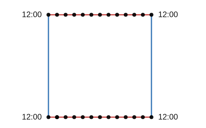
As before we can draw in the other points when the minute hand is at 12. These points correspond to 1 o’clock, 2 o’clock, 3 o’clock…
Each black dot corresponds to a time when the minute hand is at 12. Remember that each dot on the top is actually the same point as the corresponding dot on the bottom. These opposite points get glued together when we turn the square into a torus.
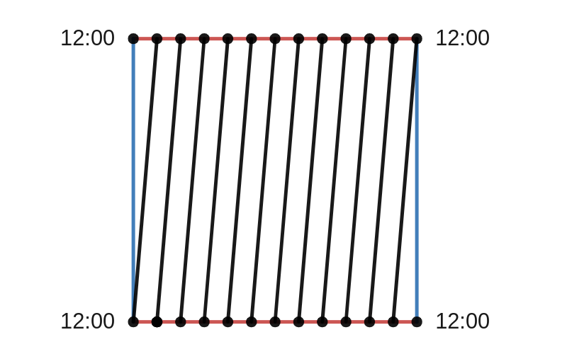
Finally we can draw in all the other times on the clock. This is the result:
Points on the black line correspond to actual times on the clock. Although it looks like there are 12 different lines, there is actually only one line once we glue the opposite sides together.
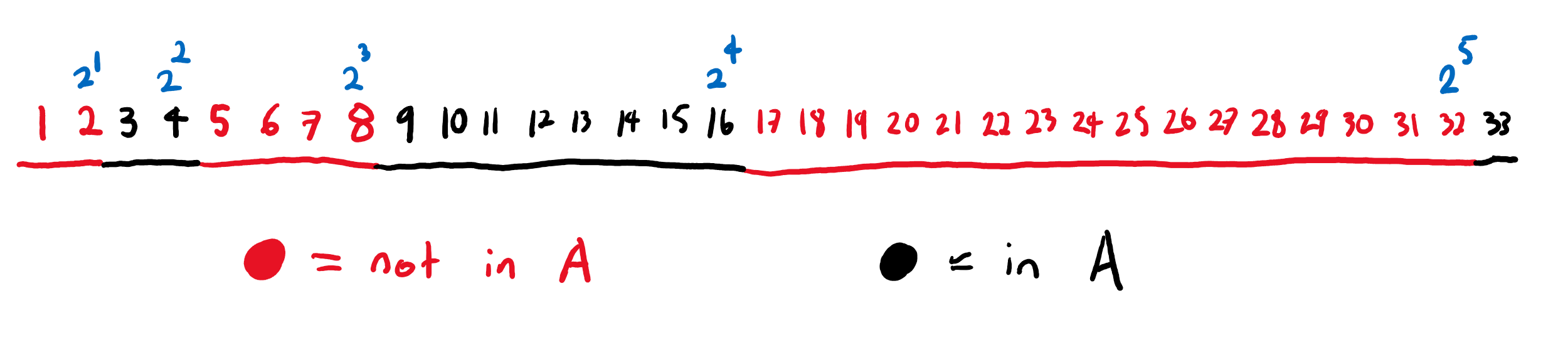
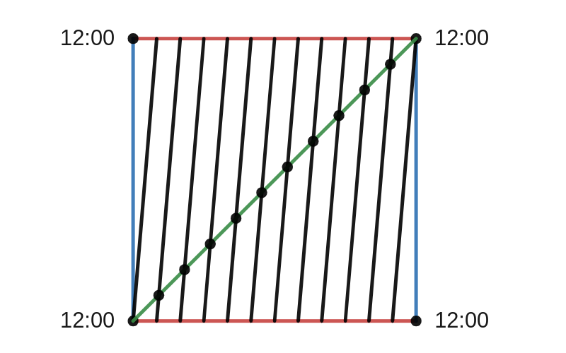
One nice thing about this picture is that it can help us answer a classic riddle. In a 12-hour cycle, how many times are the minute and hour hands on top of each other? We can answer this riddle by adding a second line to the above square. The bottom-left to top-right diagonal is the collection of all hand positions where the two hands are on top of each other. Let’s add that line in green and add the points where this new line intersects the black line.
The green line is the collection of all hand positions when the two hands are pointing in the same direction. The black points are where the green and black lines intersect each other.
The points where the green and black lines intersect are hand positions where the clock hands are directly on top of each other and which correspond to actual times. Thus we can count that there are exactly 11 times when the hands are on top of each other in a 12-hour cycle. It might look like there are 12 such times but we have to remember that the corners of the square are all the same point on the torus.
Adding the second hand
So far I have ignored the second hand on the clock. If we included the second hand, we would have three points on three different circles. The corresponding geometric object is a 3-dimensional torus. The 3-dimensional torus is what you get when you take a cube and glue together the three pairs of opposite faces (don’t worry if you have trouble visualising such a shape!).
The points on the 3-dimensional torus which correspond to actual times will again be a line that wraps around the 3-dimensional torus. You could use this line to find out how many times the three hands are all on top of each other! Let me know if you work it out.
I hope that if you’re ever asked to define a clock, you’d at least consider saying “a clock is a one-dimensional subgroup of the torus” and you could even tell them which subgroup!