I recently gave a talk on the Yang-Baxter equation. The focus of the talk was to state the connection between the Yang-Baxter equation and the braid relation. This connection comes from a system of interacting particles. In this post, I’ll go over part of my talk. You can access the full set of notes here.
Interacting particles
Imagine two particles on a line, each with a state that can be any element of a set \(\mathcal{X}\). Suppose that the only way particles can change their states is by interacting with each other. An interaction occurs when two particles pass by each other. We could define a function \(F : \mathcal{X} \times \mathcal{X} \to \mathcal{X} \times \mathcal{X}\) that describes how the states change after interaction. Specifically, if the first particle is in state \(x\) and the second particle is in state \(y\), then their states after interacting will be \(F(x,y) = (F_a(x,y), F_b(x,y))\) where \(F_a(x,y)\) is the new state of the first particle and \(F_b(x,y)\) is the state of the second particle.
Since the particles move past each other when they interact. Thus, to keep track of the whole system we need an element of \(\mathcal{X} \times \mathcal{X}\) to keep track of the states and a permutation \(\sigma \in S_2\) to keep track of the positions.
Three particles
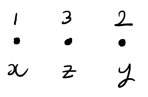
Now suppose that we have \(3\) particles labelled \(1,2,3\). As before, each particle has a state in \(\mathcal{X}\). We can thus keep track of the state of each particle with an element of \(\mathcal{X}^3\). The particles also have a position which is described by a permutation \(\sigma \in S_3\). The order the entries of \((x,y,z) \in \mathcal{X}^3\) corresponds to the labels of the particles not their positions. A possible configuration is shown below:
A possible configuration of the three particles. The above configuration is escribed as having states \((x,y,z) \in \mathcal{X}^3\) and positions \(132 \in S_3\).
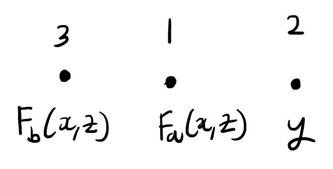
As before, the particles can interact with each other. However, we’ll now add the restriction that the particles can only interact two at a time and interacting particles must have adjacent positions. When two particles interact, they swap positions and their states change according to \(F\). The state and position of the remaining particle is unchanged. For example, in the above picture we could interact particles \(1\) and \(3\). This will produce the below configuration:
The new configuration after interacting particles \(1\) and \(3\) in the first diagram. The configuration is now described by the states \(F_{13}(x,y,z) \in \mathcal{X}^3\) and the permutation \(312 \in S_3\).
To keep track of how the states of the particles change over time we will introduce three functions from \(\mathcal{X}^3\) to \(\mathcal{X}^3\). These functions are \(F_{12},F_{13},F_{23}\). The function \(F_{ij}\) is given by applying \(F\) to the \(i,j\) coordinates of \((x,y,z)\) and acting by the identity on the remaining coordinate. In symbols,
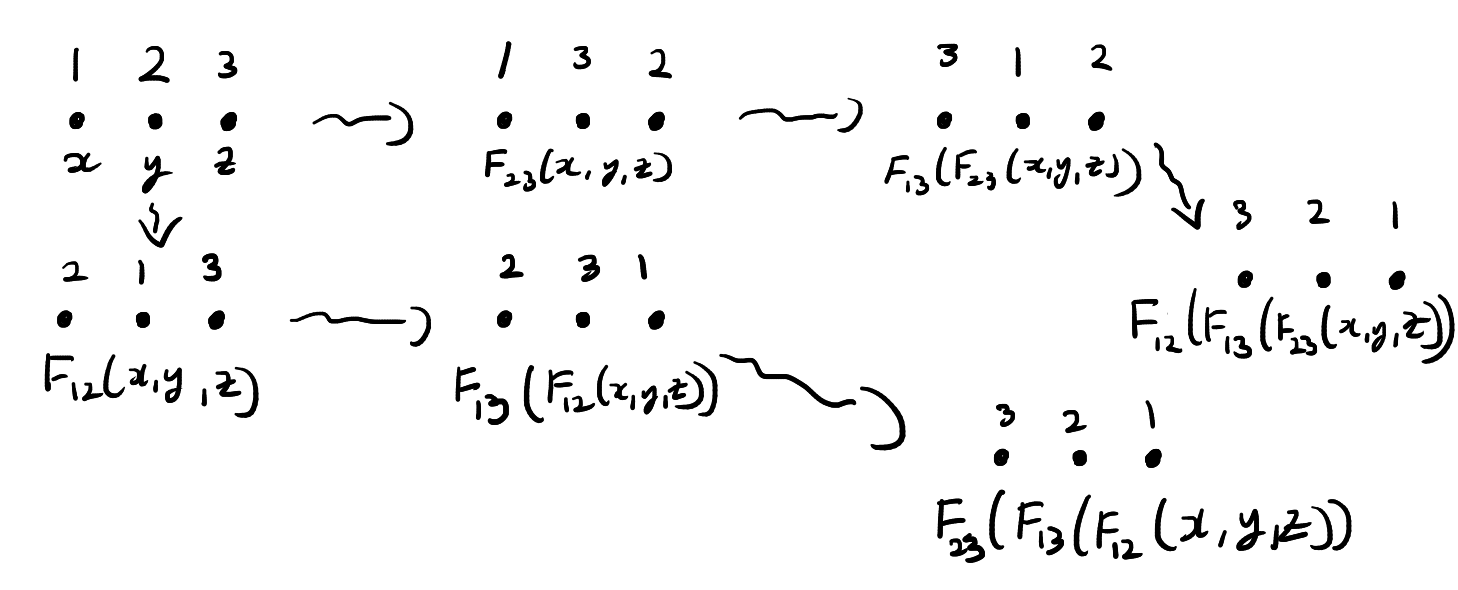
The function \(F_{ij}\) exactly describes how the states of the three particles change when particles \(i\) and \(j\) interact. Now suppose that three particles begin in position \(123\) and states \((x,y,z)\). We cannot directly interact particles \(1\) and \(3\) since they are not adjacent. We have to pass first pass one of the particles through particle \(2\). This means that there are two ways we can interact particles \(1\) and \(3\). These are illustrated below.
The two ways of passing through particle 2 to interact particles 2 and 3.
In the top chain of interactions, we first interact particles \(2\) and \(3\). In this chain of interactions, the states evolve as follows:
Note that after both of these chains of interactions the particles are in position \(321\). The function \(F\) is said to solve the Yang–Baxter equation if two chains of interactions also result in the same states.
Definition: A function \(F : \mathcal{X} \times \mathcal{X} \to \mathcal{X} \times \mathcal{X}\) is a solution to the set theoretic Yang–Baxter equation if,
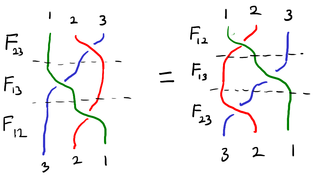
This equation can be visualized as the “braid relation” shown below. Here the strings represent the three particles and interacting two particles corresponds to crossing one string over the other.
The braid relation.
Here are some examples of solutions to the set theoretic Yang-Baxter equation,
The identity on \(\mathcal{X} \times \mathcal{X}\).
The swap map, \((x,y) \mapsto (y,x)\).
If \(f,g : \mathcal{X} \to \mathcal{X}\) commute, then the function \((x,y) \to (f(x), g(y))\) is a solution the Yang-Baxter equation.
In the full set of notes I talk about a number of extensions and variations of the Yang-Baxter equation. These include having more than three particles, allowing for the particle states to be entangle and the parametric Yang-Baxter equation.
Like my previous post, this blog is also motivated by a comment by Professor Persi Diaconis in his recent Stanford probability seminar. The seminar was about a way of “collapsing” a random walk on a group to a random walk on the set of double cosets. In this post, I’ll first define double cosets and then go over the example Professor Diaconis used to make us probabilists and statisticians more comfortable with all the group theory he was discussing.
Double cosets
Let \(G\) be a group and let \(H\) and \(K\) be two subgroups of \(G\). For each \(g \in G\), the \((H,K)\)-double coset containing \(g\) is defined to be the set
\(HgK = \{hgk : h \in H, k \in K\}\)
To simplify notation, we will simply write double coset instead of \((H,K)\)-double coset. The double coset of \(g\) can also be defined as the equivalence class of \(g\) under the relation
\(g \sim g’ \Longleftrightarrow g’ = hgk\) for some \(h \in H\) and \(g \in G\)
Like regular cosets, the above relation is indeed an equivalence relation. Thus, the group \(G\) can be written as a disjoint union of double cosets. The set of all double cosets of \(G\) is denoted by \(H\backslash G / K\). That is,
\(H\backslash G /K = \{HgK : g \in G\}\)
Note that if we take \(H = \{e\}\), the trivial subgroup, then the double cosets are simply the left cosets of \(K\), \(G / K\). Likewise if \(K = \{e\}\), then the double cosets are the right cosets of \(H\), \(H \backslash G\). Thus, double cosets generalise both left and right cosets.
Double cosets in \(S_n\)
Fix a natural number \(n > 0\). A partition of \(n\) is a finite sequence \(a = (a_1,a_2,\ldots, a_I)\) such that \(a_1,a_2,\ldots, a_I \in \mathbb{N}\), \(a_1 \ge a_2 \ge \ldots a_I > 0\) and \(\sum_{i=1}^I a_i = n\). For each partition of \(n\), \(a\), we can form a subgroup \(S_a\) of the symmetric group \(S_n\). The subgroup \(S_a\) contains all permutations \(\sigma \in S_n\) such that \(\sigma\) fixes the sets \(A_1 = \{1,\ldots, a_1\}, A_2 = \{a_1+1,\ldots, a_1 + a_2\},\ldots, A_I = \{n – a_I +1,\ldots, n\}\). Meaning that \(\sigma(A_i) = A_i\) for all \(1 \le i \le I\). Thus, a permutation \(\sigma \in S_a\) must individually permute the elements of \(A_1\), the elements of \(A_2\) and so on. This means that, in a natural way,
If we have two partitions \(a = (a_1,a_2,\ldots, a_I)\) and \(b = (b_1,b_2,\ldots,b_J)\), then we can form two subgroups \(H = S_a\) and \(K = S_b\) and consider the double cosets \(H \backslash G / K = S_a \backslash S_n / S_b\). The claim made in the seminar was that the double cosets are in one-to-one correspondence with \(I \times J\) contingency tables with row sums equal to \(a\) and column sums equal to \(b\). Before we explain this correspondence and properly define contingency tables, let’s first consider the cases when either \(H\) or \(K\) is the trivial subgroup.
Left cosets in \(S_n\)
Note that if \(a = (1,1,\ldots,1)\), then \(S_a\) is the trivial subgroup and, as noted above, \(S_a \backslash S_n / S_b\) is simply equal to \(S_n / S_b\). We will see that the cosets in \(S_n/S_b\) can be described by forgetting something about the permutations in \(S_n\).
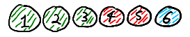
We can think of the permutations in \(S_n\) as all the ways of drawing without replacement \(n\) balls labelled \(1,2,\ldots, n\). We can think of the partition \(b = (b_1,b_2,\ldots,b_J)\) as a colouring of the \(n\) balls by \(J\) colours. We colour balls \(1,2,\ldots, b_1\) by the first colour \(c_1\), then we colour \(b_1+1,b_1+2,\ldots, b_1+b_2\) the second colour \(c_2\) and so on until we colour \(n-b_J+1, n-b_J+2,\ldots, n\) the final colour \(c_J\). Below is an example when \(n\) is equal to 6 and \(b = (3,2,1)\).
The first three balls are coloured green, the next two are coloured red and the last ball is coloured blue.
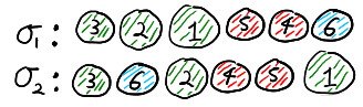
Note that a permutation \(\sigma \in S_n\) is in \(S_b\) if and only if we draw the balls by colour groups, i.e. we first draw all the balls with colour \(c_1\), then we draw all the balls with colour \(c_2\) and so on. Thus, continuing with the previous example, the permutation \(\sigma_1\) below is in \(S_b\) but \(\sigma_2\) is not in \(S_b\).
The permutation \(\sigma_1\) is in \(S_b\) because the colours are in their original order but \(\sigma_1\) is not in \(S_b\) because the colours are rearranged.
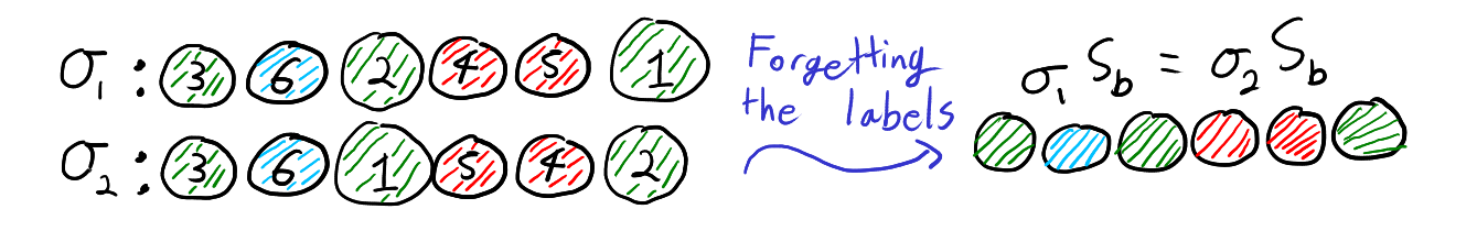
It turns out that we can think of the cosets in \(S_n \setminus S_b\) as what happens when we “forget” the labels \(1,2,\ldots,n\) and only remember the colours of the balls. By “forgetting” the labels we mean only paying attention to the list of colours. That is for all \(\sigma_1,\sigma_2 \in S_n\), \(\sigma_1 S_b = \sigma_2 S_b\) if and only if the list of colours from the draw \(\sigma_1\) is the same as the list of colours from the draw \(\sigma_2\). Thus, the below two permutations define the same coset of \(S_b\)
When we forget the labels and only remember the colours, the permutations \(\sigma_1\) and \(\sigma_2\) look the same and thus are in the same left coset of \(S_b\).
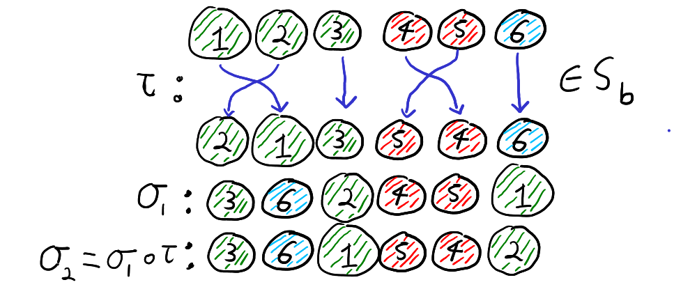
To see why this is true, note that \(\sigma_1 S_b = \sigma_2 S_b\) if and only if \(\sigma_2 = \sigma_1 \circ \tau\) for some \(\tau \in S_b\). Furthermore, \(\tau \in S_b\) if and only if \(\tau\) maps each colour group to itself. Recall that function composition is read right to left. Thus, the equation \(\sigma_2 = \sigma_1 \circ \tau\) means that if we first relabel the balls according to \(\tau\) and then draw the balls according to \(\sigma_1\), then we get the result as just drawing by \(\sigma_2\). That is, \(\sigma_2 = \sigma_1 \circ \tau\) for some \(\tau \in S_b\) if and only if drawing by \(\sigma_2\) is the same as first relabelling the balls within each colour group and then drawing the balls according to \(\sigma_1\). Thus, \(\sigma_1 S_b = \sigma_2 S_b\), if and only if when we forget the labels of the balls and only look at the colours, \(\sigma_1\) and \(\sigma_2\) give the same list of colours. This is illustrated with our running example below.
If we permute the balls according to \(\tau \in S_b\) and the draw according to \(\sigma_1\), then the resulting draw is the same as if we had not permuted and drawn according to \(\sigma_2\). That is, \(\sigma_2 = \sigma_1 \circ \tau\).
Right cosets of \(S_n\)
Typically, the subgroup \(S_a\) is not a normal subgroup of \(S_n\). This means that the right coset \(S_a \sigma\) will not equal the left coset \(\sigma S_a\). Thus, colouring the balls and forgetting the labelling won’t describe the right cosets \(S_a \backslash S_n\). We’ll see that a different type of forgetting can be used to describe \(S_a \backslash S_n = \{S_a\sigma : \sigma \in S_n\}\).
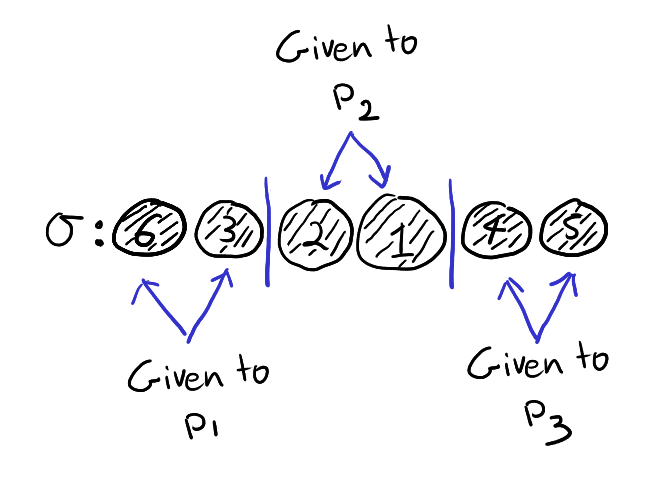
Fix a partition \(a = (a_1,a_2,\ldots,a_I)\) and now, instead of considering \(I\) colours, think of \(I\) different people \(p_1,p_2,\ldots,p_I\). As before, a permutation \(\sigma \in S_n\) can be thought of drawing \(n\) balls labelled \(1,\ldots,n\) without replacement. We can imagine giving the first \(a_1\) balls drawn to person \(p_1\), then giving the next \(a_2\) balls to the person \(p_2\) and so on until we give the last \(a_I\) balls to person \(p_I\). An example with \(n = 6\) and \(a = (2,2,2)\) is drawn below.
Person \(p_1\) receives the ball labelled by 6 followed by the ball labelled 3, person \(p_2\) receives ball 2 and then ball 1 and finally person \(p_3\) receives ball 4 followed by ball 5.
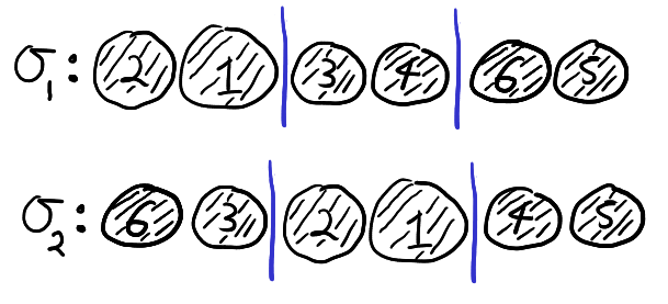
Note that \(\sigma \in S_a\) if and only if person \(p_i\) receives the balls with labels \(\sum_{k=0}^{i-1}a_k+1,\sum_{k=0}^{i-1}a_k+2,\ldots, \sum_{k=0}^i a_k\) in any order. Thus, in the below example \(\sigma_1 \in S_a\) but \(\sigma_2 \notin S_a\).
When the balls are drawn according to \(\sigma_1\), person \(p_i\) receives the balls with labels \(2i-1\) and \(2i\), and thus \(\sigma_1 \in S_a\). On the other hand, if the balls are drawn according to \(\sigma_2\), the people receive different balls and thus \(\sigma_2 \notin S_a\).
It turns out the cosets \(S_a \backslash S_n\) are exactly determined by “forgetting” the order in which each person \(p_i\) received their balls and only remembering which balls they received. Thus, the two permutation below belong to the same coset in \(S_a \backslash S_n\).
When we forget the order in which each person receive their balls, the permutations \(\sigma_1\) and \(\sigma_2\) become the same and thus \(S_a \sigma_1 = S_a \sigma_2\). Note that if we coloured the balls according to the permutation \(a = (a_1,\ldots,a_I)\), then we could see that \(\sigma_1 S_a \neq \sigma_2 S_a\).
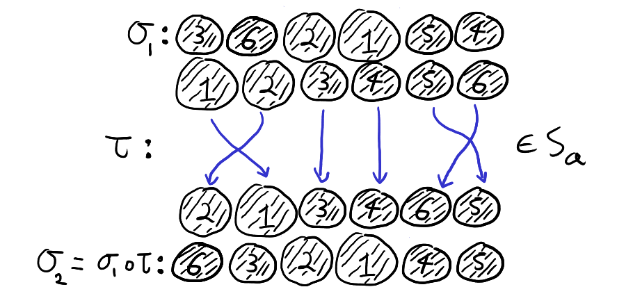
To see why this is true in general, consider two permutations \(\sigma_1,\sigma_2\). The permutations \(\sigma_1,\sigma_2\) result in each person \(p_i\) receiving the same balls if and only if after \(\sigma_1\) we can apply a permutation \(\tau\) that fixes each subset \(A_i = \left\{\sum_{k=0}^{i-1}a_k+1,\ldots, \sum_{k=0}^i a_k\right\}\) and get \(\sigma_2\). That is, \(\sigma_1\) and \(\sigma_2\) result in each person \(p_i\) receiving the same balls if and only if \(\sigma_2 = \tau \circ \sigma_1\) for some \(\tau \in S_a\). Thus, \(\sigma_1,\sigma_2\) are the same after forgetting the order in which each person received their balls if and only if \(S_a \sigma_1 = S_a \sigma_2\). This is illustrated below,
If we first draw the balls according to \(\sigma_1\) and then permute the balls according to \(\tau\), then the resulting draw is the same as if we had drawn according to \(\sigma_2\) and not permuted afterwards. That is, \(\sigma_2 = \tau \circ \sigma_1 \).
We can thus see why \(S_a \backslash S_n \neq S_n / S_a\). A left coset \(\sigma S_a\) correspond to pre-composing \(\sigma\) with elements of \(S_a\) and a right cosets \(S_a\sigma\) correspond to post-composing \(\sigma\) with elements of \(S_a\).
Contingency tables
With the last two sections under our belts, describing the double cosets \(S_a \backslash S_n / S_b\) is straight forward. We simply have to combine our two types of forgetting. That is, we first colour the \(n\) balls with \(J\) colours according to \(b = (b_1,b_2,\ldots,b_J)\). We then draw the balls without replace and give the balls to \(I\) different people according \(a = (a_1,a_2,\ldots,a_I)\). We then forget both the original labels and the order in which each person received their balls. That is, we only remember the number of balls of each colour each person receives. Describing the double cosets by “double forgetting” is illustrated below with \(a = (2,2,2)\) and \(b = (3,2,1)\).
The permutations \(\sigma_1\) and \(\sigma_2\) both result in person \(p_1\) receiving one green ball and one blue ball. The two permutations also results in \(p_2\) and \(p_3\) both receiving one green ball and one red ball. Thus, \(\sigma_1\) and \(\sigma_2\) are both in the same \((S_a,S_b)\)-double coset. Note however that \(\sigma_1 S_b \neq \sigma_2 S_b\) and \(S_a\sigma_1 \neq S_a \sigma_2\).
The proof that double forgetting does indeed describe the double cosets is simply a combination of the two arguments given above. After double forgetting, the number of balls given to each person can be recorded in an \(I \times J\) table. The \(N_{ij}\) entry of the table is simply the number of balls person \(p_i\) receives of colour \(c_j\). Two permutations are the same after double forgetting if and only if they produce the same table. For example, \(\sigma_1\) and \(\sigma_2\) above both produce the following table
Green (\(c_1\))
Red (\(c_2\))
Blue (\(c_3\))
Total
Person \(p_1\)
1
0
1
2
Person \(p_2\)
1
1
0
2
Person \(p_3\)
1
1
0
2
Total
3
2
1
6
By the definition of how the balls are coloured and distributed to each person we must have for all \(1 \le i \le I\) and \(1 \le j \le J\)
\(\sum_{j=1}^J N_{ij} = a_i \) and \(\sum_{i=1}^I N_{ij} = b_j\)
An \(I \times J\) table with entries \(N_{ij} \in \{0,1,2,\ldots\}\) satisfying the above conditions is called a contingency table. Given such a contingency table with entries \(N_{ij}\) where the rows sum to \(a\) and the columns sum to \(b\), there always exists at least one permutation \(\sigma\) such that \(N_{ij}\) is the number of balls received by person \(p_i\) of colour \(c_i\). We have already seen that two permutations produce the same table if and only if they are in the same double coset. Thus, the double cosets \(S_a \backslash S_n /S_b\) are in one-to-one correspondence with such contingency tables.
The hypergeometric distribution
I would like to end this blog post with a little bit of probability and relate the contingency tables above to the hyper geometric distribution. If \(a = (m, n-m)\) for some \(m \in \{0,1,\ldots,n\}\), then the contingency tables described above have two rows and are determined by the values \(N_{11}, N_{12},\ldots, N_{1J}\) in the first row. The numbers \(N_{1j}\) are the number of balls of colour \(c_j\) the first person receives. Since the balls are drawn without replacement, this means that if we put the uniform distribution on \(S_n\), then the vector \(Y=(N_{11}, N_{12},\ldots, N_{1J})\) follows the multivariate hypergeometric distribution. Thus, if we have a random walk on \(S_n\) that quickly converges to the uniform distribution on \(S_n\), then we could use the double cosets to get a random walk that converges to the multivariate hypergeometric distribution (although there are smarter ways to do such sampling).
Something very exciting this afternoon. Professor Persi Diaconis was presenting at the Stanford probability seminar and the field with one element made an appearance. The talk was about joint work with Mackenzie Simper and Arun Ram. They had developed a way of “collapsing” a random walk on a group to a random walk on the set of double cosets. As an illustrative example, Persi discussed a random walk on \(GL_n(\mathbb{F}_q)\) given by multiplication by a random transvection (a map of the form \(v \mapsto v + ab^Tv\), where \(a^Tb = 0\)).
The Bruhat decomposition can be used to match double cosets of \(GL_n(\mathbb{F}_q)\) with elements of the symmetric group \(S_n\). So by collapsing the random walk on \(GL_n(\mathbb{F}_q)\) we get a random walk on \(S_n\) for all prime powers \(q\). As Professor Diaconis said, you can’t stop him from taking \(q \to 1\) and asking what the resulting random walk on \(S_n\) is. The answer? Multiplication by a random transposition. As pointed sets are vector spaces over the field with one element and the symmetric groups are the matrix groups, this all fits with what’s expected of the field with one element.
This was just one small part of a very enjoyable seminar. There was plenty of group theory, probability, some general theory and engaging examples.
Update: I have written another post about some of the group theory from the seminar! You can read it here: Double cosets and contingency tables.
In July 2020 I submitted my honours thesis which was titled “Commuting in Groups” and supervised by Professor Anthony Licata. You can read the abstract below and the full thesis here.
Abstract
In this thesis, we study four different classes of groups coming from geometric group theory. Each of these classes are defined in terms of fellow traveller conditions. First we study automatic groups and show that such groups have a solvable word problem. We then study hyperbolic groups and show that a group is hyperbolic if and only if it is strongly geodesically automatic. We also show that a group is hyperbolic if and only if it has a divergence function. We next study combable groups and examine some examples of groups that are combable but not automatic. Finally we introduce biautomatic groups. We show that biautomatic groups have a solvable conjugacy problem and that many nilpotent groups cannot be subgroups of biautomatic groups. Finally we introduce Artin groups of finite type and show that all such groups are biautomatic.
In the previous blog post we observed that if a polynomial \(g\) could be written as a sum \(\sum_{i=1}^n h_i^2\) where each \(h_i\) is a polynomial, then \(g\) must be non-negative. We then asked if the converse was true. That is, if \(g\) is a non-negative polynomial, can \(g\) be written a sum of squares of polynomials? As we saw, a positive answer to this question would allow us to optimize a polynomial function \(f\) by looking at the values of \(\lambda\) such that \(g = f – \lambda\) can be written as a sum of squares.
Unfortunately, as we shall see, not all non-negative polynomials can be written as sums of squares.
The Motzkin Polynomial
The Motzkin polynomial is a two variable polynomial defined by
\(g(x,y) = x^4y^2 +x^2y^4-3x^2y^2+1\).
We wish to prove two things about this polynomial. The first claim is that \(g(x,y) \ge 0\) for all \(x,y \in \mathbb{R}\) and the second claim is that \(g\) cannot be written as a sum of squares of polynomials. To prove the first claim we will use the arithmetic mean geometric mean inequality. This inequality states that for all \(n \in \mathbb{N}\) and all \(a_1,a_2,\ldots, a_n \ge 0\), we have that
Simplifying the left hand side and multiplying both sides by \(3\) gives that
\(3x^2 y^2 \le x^4 y^2 + y^2 x^4 + 1\).
Since our Motzkin polynomial \(g\) is given by \(g(x,y) = x^4 y^2 + y^2 x^2 – 3x^2 y^2 +1\), the above inequality is equivalent to \(g(x,y) \ge 0\).
Newton Polytopes
Thus we have shown that the Motzkin polynomial is non-negative. We now wish to show that it is not a sum of squares. To do this we will first have to define the Newton polytope of a polynomial. If our polynomial \(f\) has \(n\) variables, then the Newton polytope of \(f\), denoted \(N(f)\) is a convex subset of \(\mathbb{R}^n\). To define \(N(f)\) we associate a point in \(\mathbb{R}^n\) to each term of the polynomial \(f\) based on the degree of each variable. For instance the term \(3x^2y^4\) is assigned the point \((2,4) \in \mathbb{R}^2\) and the term \(4xyz^3\) is assigned the point \((1,1,3) \in \mathbb{R}^2\). Note that the coefficients of the term don’t affect this assignment.
We then define \(N(f)\) to be the convex hull of all points assigned to terms of the polynomial \(f\). For instance if \(f(x,y) = x^4y^3+5x^3y – 7y^3+8\), then the Newton polytope of \(f\) is the following subset of \(\mathbb{R}^2\).
Note again that changing the non-zero coefficients of the polynomial \(f\) does not change \(N(f)\).
Now suppose that our polynomial is a sum of squares, that is \(f = \sum_{i=1}^n h_i^2\). It turns out the the Newton polytope of \(f\) can be defined in terms of the Newton polytopes of \(h_i\). In particular we have that \(N(f) =2X\) where \(X\) is the convex hull of the union of \(N(h_i)\) for \(i = 1,\ldots, n\).
To see why this is true, note that if \(a\) and \(b\) are the points corresponding to two terms \(p\) and \(q\), then \(a+b\) corresponds to \(pq\). Thus we can see that every term of \(f\) corresponds to a point that can be written as \(a+b\) for some \(a,b \in N(h_i)\). It follows that \(N(f) \subseteq 2X\).
Conversely note that if we have terms \(p, q, r\) corresponding to points \(a,b, c\) and \(pq = r^2\), then \(a+b = 2c\). It follows that if \(c\) is a vertex in \(X\) corresponding to the term \(r\) in some polynomial \(h_i\) and \(p,q\) are two terms in a polynomial \(h_j\) such that \(pq = r^2\), then \(p=q=r\). This is because if \(r\) was not equal to either \(p\) or \(q\), then the point \(c\) would not be a vertex and would instead lie on the line between the points assigned to \(p\) and \(q\).
It follows that if \(c\) is a vertex of \(X\) with corresponding term \(r\), then \(r^2\) appears with a positive coefficient in \(f = \sum_{i=1}^n h_i\). It follows that \(2X \subseteq N(f)\) and so \(2X = N(f)\).
Not a sum of squares
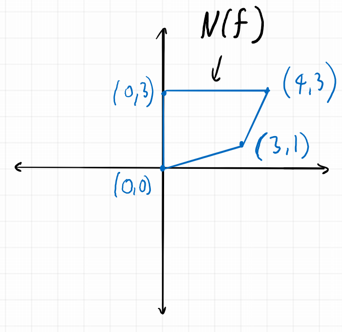
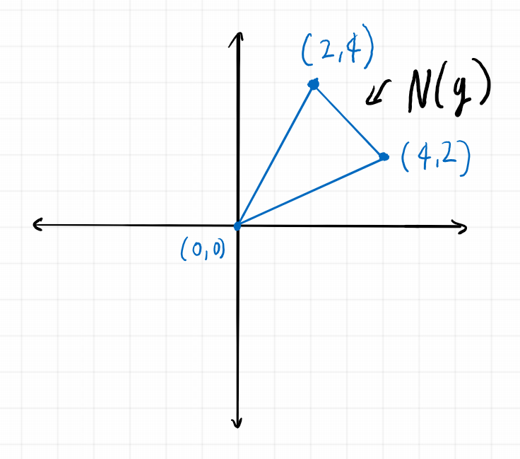
Let’s now take another look at the Motzkin polynomial which is defined to be
\(g(x,y) = x^4y^2 + x^2 y^4 – 3x^2y^2 + 1\).
Thus the Newton polytope of \(g\) has corners \((4,2), (2,4), (0,0)\) and looks like this
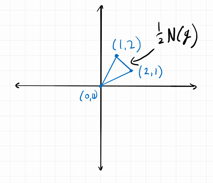
Thus if the Motzkin polynomial was a sum of squares \(g = \sum_{i=1}^n h_i^2\), then the Newton polytope of each \(h_i\) must be contained in \(\frac{1}{2}N(g)\). Now \(\frac{1}{2}N(g)\) looks like this
The only integer points contained in \(\frac{1}{2}N(g)\) are \((0,0), (1,1), (1,2)\) and \((2,1)\). Thus each \(h_i\) must be equal to \(h_i(x,y) = a_i x^2 y+b_i xy^2 + c_i xy + d_i\). If we square this polynomial we see that the coefficient of \(x^2 y^2 \) is \(c_i^2\). Thus the coefficient of \(x^2y^2 \) in \(\sum_{i=1}^n h_i^2\) must be \(c_1^2+c_2^2+\ldots +c_n^2 \ge 0\). But in the Motzkin polynomial, \(x^2y^2\) has coefficient \(-3\).
Thus the Motzkin polynomial is a concrete example of a non-negative polynomial that is not a sum of squares.
References
As stated in the first part of this series, these two blog posts are based off conversations I had with Abhishek Bhardwaj last year. I also used these slides to remind myself why the Motzkin polynomial is not a sum of squares.