Author: michaelnhowes

  • Leverages Scores

    I am very excited to be writing a blog post again – it has been nearly a year! This post marks a new era for the blog. In September I started a statistics PhD at Stanford University. I am really enjoying my classes and I am learning a lot. I might have to change the name of the blog soon but for now let’s stick with “Maths to Share” although you will undoubtedly see more and more statistics here.

    Today I would like to talk about leverages scores. Leverages scores are a way to quantify how sensitive a model is and they can be used to explain the different behaviour in these two animations

    Linear Models

    I recently learnt about leverage scores in the applied statistics course STATS 305A. This course is all about the linear model. In the linear model we assume with have \(n\) data points \((x_i,y_i)\) where \(x_i\) is a vector in \(\mathbb{R}^d\) and \(y_i\) is a number in \(\mathbb{R}\). We model \(y_i\) as a linear function of \(x_i\) plus noise. That is we assume \(y_i = x_i^T\beta + \varepsilon_i\), where \(\beta \in \mathbb{R}^d\) is a unknown vector of coefficients and \(\varepsilon_i\) is a random variable with mean \(0\) and variance \(\sigma^2\). We also require that for \(i \neq j\), the random variable \(\varepsilon_i\) is uncorrelated with \(\varepsilon_j\).

    We can also write this as a matrix equation. Define \(y\) to be the vector with entries \(y_i\) and define \(X\) to be the matrix with rows \(x_i^T\), that is

    \(y = \begin{bmatrix} y_1\\ y_2 \\ \vdots \\ y_n \end{bmatrix} \in \mathbb{R}^n\) and \(X = \begin{bmatrix} -x_1^T-\\-x_2^T-\\ \vdots \\ -x_n^T-\end{bmatrix} \in \mathbb{R}^{n \times d}.\)

    Then our model can be rewritten as

    \(y = X\beta + \varepsilon,\)

    where \(\varepsilon \in \mathbb{R}^n\) is a random vector with mean \(0\) and covariance matrix \(\sigma^2 I_n\). To simplify calculations we will assume that \(X\) contains an intercept term. This means that the first column of \(X\) consists of all 1’s.

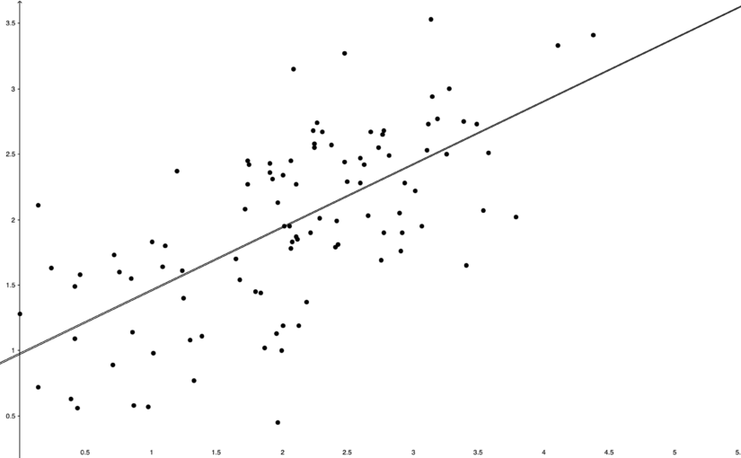
    In the two animations at the start of this post we have two nearly identical data sets. The data sets are an example of simple regression when each vector \(x_i\) is of the form \((1,z_i)\) where \(z_i\) is a number. The values \(z_i\) are on the horizontal axis and the values \(y_i\) are on the vertical axis.

    Estimating the coefficients

    In the linear model we wish to estimate the parameter \(\beta\) which contains the coefficients of our model. That is, given a sample \((y_i,x_i)_{i=1}^n\), we wish to construct a vector \(\widehat{\beta}\) which approximates the true parameter \(\beta\). In ordinary least square regression we choose \(\widehat{\beta}\) to be the vector \(b \in \mathbb{R}^d\) that minimizes the quantity

    \(\sum_{i=1}^n (x_i^T b – y_i)^2=\left \Vert Xb – y \right \Vert_2^2\).

    Differentiating with respect to \(b\) and setting the derivative equal to \(0\) shows that \(\widehat{\beta}\) is a solution to the normal equations:

    \(X^TXb = X^T y.\)

    We will assume that the matrix \(X^TX\) is invertible. In this case then the normal equations have a unique solution \(\widehat{\beta} = (X^TX)^{-1}X^T y\).

    Now that we have our estimate \(\widehat{\beta}\), we can do prediction. If we are given a new value \(x’ \in \mathbb{R}^d\) we would use \(x’^T\widehat{\beta}\) to predict the corresponding value of \(y’\). This was how the straight lines in the two animations were calculated.

    We can also calculate the model’s predicted values for the data \(x_i\) that we used to fit the model. These are denoted by \(\widehat{y}\). Note that

    \(\widehat{y} = X\widehat{\beta} = X(X^TX)^{-1}X^Ty = Hy,\)

    where \(H = X(X^TX)^{-1}X^T\) is called the hat matrix for the model (since it puts the hat \(\widehat{ }\) on \(y\).

    Leverage scores

    We are now ready to talk about leverage scores and the two animations. For reference, here they are again:

    In both animations the stationary line corresponds to an estimator \(\widehat{\beta}\) that was calculated using only the black data points. The red points are new data points with different \(x\) values and varying \(y\) values. The moving line corresponds to an estimator \(\widehat{\beta}\) calculated using the red data point as well as all the black points. We can see immediately that if the red point is far away from the “bulk” of the other \(x\) points, then the moving line is a lot more sensitive to the \(y\) value of the red point.

    The leverage score of a data point \((x_i,y_i)\) is defined to be \(\frac{\partial \widehat{y}_i}{\partial y_i}.\) That is, the leverage score tells us how much does the prediction \(\widehat{y}_i\) change if we change \(y_i\).

    Since \(\widehat{y} = Hy\), the leverage score of \((x_i,y_i)\) is \(H_{ii}\), the \(i^{th}\) diagonal element of the hat matrix \(H\). The idea is that if a data point \((x_i,y_i)\) has a large leverage score, then the model is more sensitive to changes in that value of \(y_i\).

    This can be seen in a leave one out calculation. This calculation tells us what we should expect if we make a leave-one-out model – a model that uses all the data points apart from one. In our animations, this corresponds to the stationary line.

    The leave one out calculation says that the predicted value using all the data is always between the true value and the predicted value from the leave-one-out model. In our animations this can be seen by noting that the moving line (the full model) is always between the red point (the true value) and the stationary line (the leave-one-out model).

    Furthermore the leverage score tells us exactly how close the predicted value is to the true value. We can see that the moving line is much closer to the red dot in the high leverage example on the right than the low leverage example on the left.

    Mahalanobis distance

    We now know that the two animations are showing the sensitivity of a model to two different data points. We know that a model is more sensitive to point with high leverage than to points with low leverage. We still haven’t spoken about why some point have higher leverage and why the point on the right has higher leverage.

    It turns out that leverage score are measuring how far away a data point is from the “bulk” of the other \(x_i\)’s. More specifically in a one dimensional example like what we have in the animations

    \(H_{ii} = \frac{1}{n}\left(\frac{1}{S^2}(x_i-\bar{x})^2+1\right),\)

    where \(n\) is the number of data points, \(\bar{x} = \frac{1}{n}\sum_{j=1}^n x_j\) is the sample mean and \(S^2 = \frac{1}{n}\sum_{j=1}^n (x_j-\bar{x})^2\) is the sample variance. Thus high leverage scores correspond to points that are far away from the centre of our data \(x_i\). In higher dimensions a similar result holds if we measure distance using Mahalanobis distance.

    The mean of the black data points is approximately 2 and so we can now see why the second point has higher leverage. The two animations were made in Geogebra. You can play around with them here and here.

  • Commuting in Groups

    In July 2020 I submitted my honours thesis which was titled “Commuting in Groups” and supervised by Professor Anthony Licata. You can read the abstract below and the full thesis here.

    Abstract

    In this thesis, we study four different classes of groups coming from geometric group theory. Each of these classes are defined in terms of fellow traveller conditions. First we study automatic groups and show that such groups have a solvable word problem. We then study hyperbolic groups and show that a group is hyperbolic
    if and only if it is strongly geodesically automatic. We also show that a group is hyperbolic if and only if it has a divergence function. We next study combable groups and examine some examples of groups that are combable but not automatic. Finally we introduce biautomatic groups. We show that biautomatic groups have a solvable conjugacy problem and that many nilpotent groups cannot be subgroups of biautomatic groups. Finally we introduce Artin groups of finite type and show that all such groups are biautomatic.

  • Sums of Squares – Part 2: Motzkin

    In the previous blog post we observed that if a polynomial \(g\) could be written as a sum \(\sum_{i=1}^n h_i^2\) where each \(h_i\) is a polynomial, then \(g\) must be non-negative. We then asked if the converse was true. That is, if \(g\) is a non-negative polynomial, can \(g\) be written a sum of squares of polynomials? As we saw, a positive answer to this question would allow us to optimize a polynomial function \(f\) by looking at the values of \(\lambda\) such that \(g = f – \lambda\) can be written as a sum of squares.

    Unfortunately, as we shall see, not all non-negative polynomials can be written as sums of squares.

    The Motzkin Polynomial

    The Motzkin polynomial is a two variable polynomial defined by

    \(g(x,y) = x^4y^2 +x^2y^4-3x^2y^2+1\).

    We wish to prove two things about this polynomial. The first claim is that \(g(x,y) \ge 0\) for all \(x,y \in \mathbb{R}\) and the second claim is that \(g\) cannot be written as a sum of squares of polynomials. To prove the first claim we will use the arithmetic mean geometric mean inequality. This inequality states that for all \(n \in \mathbb{N}\) and all \(a_1,a_2,\ldots, a_n \ge 0\), we have that

    \(\left(a_1a_2\ldots a_n\right)^{1/n} \le \frac{a_1+a_2+\ldots+a_n}{n}.\)

    We will apply this inequality with \(n = 3\), \(a_1 = x^4 y^2\), \(a_2 = x^2 y^4\) and \(a_3 = 1\). This gives that

    \(\left(x^4 y^2 x^2 y^4 1\right)^\frac{1}{3} \le \frac{x^4 y^2 + y^2 x^4 +1 }{3}\).

    Simplifying the left hand side and multiplying both sides by \(3\) gives that

    \(3x^2 y^2 \le x^4 y^2 + y^2 x^4 + 1\).

    Since our Motzkin polynomial \(g\) is given by \(g(x,y) = x^4 y^2 + y^2 x^2 – 3x^2 y^2 +1\), the above inequality is equivalent to \(g(x,y) \ge 0\).

    Newton Polytopes

    Thus we have shown that the Motzkin polynomial is non-negative. We now wish to show that it is not a sum of squares. To do this we will first have to define the Newton polytope of a polynomial. If our polynomial \(f\) has \(n\) variables, then the Newton polytope of \(f\), denoted \(N(f)\) is a convex subset of \(\mathbb{R}^n\). To define \(N(f)\) we associate a point in \(\mathbb{R}^n\) to each term of the polynomial \(f\) based on the degree of each variable. For instance the term \(3x^2y^4\) is assigned the point \((2,4) \in \mathbb{R}^2\) and the term \(4xyz^3\) is assigned the point \((1,1,3) \in \mathbb{R}^2\). Note that the coefficients of the term don’t affect this assignment.

    We then define \(N(f)\) to be the convex hull of all points assigned to terms of the polynomial \(f\). For instance if \(f(x,y) = x^4y^3+5x^3y – 7y^3+8\), then the Newton polytope of \(f\) is the following subset of \(\mathbb{R}^2\).

    Note again that changing the non-zero coefficients of the polynomial \(f\) does not change \(N(f)\).

    Now suppose that our polynomial is a sum of squares, that is \(f = \sum_{i=1}^n h_i^2\). It turns out the the Newton polytope of \(f\) can be defined in terms of the Newton polytopes of \(h_i\). In particular we have that \(N(f) =2X\) where \(X\) is the convex hull of the union of \(N(h_i)\) for \(i = 1,\ldots, n\).

    To see why this is true, note that if \(a\) and \(b\) are the points corresponding to two terms \(p\) and \(q\), then \(a+b\) corresponds to \(pq\). Thus we can see that every term of \(f\) corresponds to a point that can be written as \(a+b\) for some \(a,b \in N(h_i)\). It follows that \(N(f) \subseteq 2X\).

    Conversely note that if we have terms \(p, q, r\) corresponding to points \(a,b, c\) and \(pq = r^2\), then \(a+b = 2c\). It follows that if \(c\) is a vertex in \(X\) corresponding to the term \(r\) in some polynomial \(h_i\) and \(p,q\) are two terms in a polynomial \(h_j\) such that \(pq = r^2\), then \(p=q=r\). This is because if \(r\) was not equal to either \(p\) or \(q\), then the point \(c\) would not be a vertex and would instead lie on the line between the points assigned to \(p\) and \(q\).

    It follows that if \(c\) is a vertex of \(X\) with corresponding term \(r\), then \(r^2\) appears with a positive coefficient in \(f = \sum_{i=1}^n h_i\). It follows that \(2X \subseteq N(f)\) and so \(2X = N(f)\).

    Not a sum of squares

    Let’s now take another look at the Motzkin polynomial which is defined to be

    \(g(x,y) = x^4y^2 + x^2 y^4 – 3x^2y^2 + 1\).

    Thus the Newton polytope of \(g\) has corners \((4,2), (2,4), (0,0)\) and looks like this

    Thus if the Motzkin polynomial was a sum of squares \(g = \sum_{i=1}^n h_i^2\), then the Newton polytope of each \(h_i\) must be contained in \(\frac{1}{2}N(g)\). Now \(\frac{1}{2}N(g)\) looks like this

    The only integer points contained in \(\frac{1}{2}N(g)\) are \((0,0), (1,1), (1,2)\) and \((2,1)\). Thus each \(h_i\) must be equal to \(h_i(x,y) = a_i x^2 y+b_i xy^2 + c_i xy + d_i\). If we square this polynomial we see that the coefficient of \(x^2 y^2 \) is \(c_i^2\). Thus the coefficient of \(x^2y^2 \) in \(\sum_{i=1}^n h_i^2\) must be \(c_1^2+c_2^2+\ldots +c_n^2 \ge 0\). But in the Motzkin polynomial, \(x^2y^2\) has coefficient \(-3\).

    Thus the Motzkin polynomial is a concrete example of a non-negative polynomial that is not a sum of squares.

    References

    As stated in the first part of this series, these two blog posts are based off conversations I had with Abhishek Bhardwaj last year. I also used these slides to remind myself why the Motzkin polynomial is not a sum of squares.

  • Sums of Squares – Part 1: Optimization

    About a year ago I had the pleasure of having a number of conversations with Abhishek Bhardwaj about the area of mathematics his PhD is on. This pair of posts is based on the fond memories I have of these conversations. Part two can be found here.

    Optimization and Summing Squares

    Optimization is a huge area of both pure and applied mathematics. Many questions and problems can be reduced to finding the minimum or maximum value of some function. That is we have a function \(f : \mathbb{R}^n \to \mathbb{R}\) and we wish to find the number \(\lambda\) such that

    \(\lambda = \min \{ f(x_1,\ldots, x_n) \mid (x_1,\ldots, x_n) \in \mathbb{R}^n \}\),

    or

    \(\lambda = \max \{ f(x_1,\ldots, x_n) \mid (x_1,\ldots, x_n) \in \mathbb{R}^n \}\).

    By considering the function \(-f\) we can reduce finding the maximum of \(f\) to finding the minimum of another function. Minimizing a function isn’t always easy. Even when the function \(f\) is a relative simple function such as a polynomial, it can be a very difficult problem.

    A different way of thinking about the problem of minimizing the function \(f\), is to instead think about the function \(f – \lambda\) were \(\lambda\) is a real number. The minimum of \(f\) is the largest value of \(\lambda\) such that the function \(f – \lambda\) is non-negative for all values \(x \in \mathbb{R}^n\). Thus we have a reduced our optimization problem into the problem of working out for which values of \(\lambda\) is the function \(f-\lambda\) non-negative.

    An example

    Suppose our function \(f\) was the following function that takes in two variables

    \(f(x,y) = 2x^2 + 4y^2-4xy-4x+4y+7\).

    To minimize this function we can look at the function \(g = f – \lambda\) which is equal to

    \(g(x,y) = 2x^2 + 4y^2-4xy-4x+4y+7 – \lambda\).

    We wish to work for which values of \(\lambda\) is this function \(g\) non-negative. By doing the following algebraic manipulations we can rewrite \(g\) like so

    \(g(x,y) = (x^2-2x+1)+(x^2+4y^2+1-4xy-2x+4y)+5-\lambda \),

    which is in turn equal to

    \(g(x,y) = (x-1)^2+(-x+2y+1)^2 +(5-\lambda)\)

    Since \((x-1)^2\) and \((-x+2y+1)^2\) are both squares of real numbers, they are both non-negative. Furthermore at the point \((x,y) = (1,0)\), we have that \((x-1)^2+(-x+2y+1)^2=0\). Thus \(g\) is non-negative if and only if \((5-\lambda) \ge 0\), that is if and only if \(\lambda \le 5\). Thus we can conclude that the minimum of \(f\) is \(5\).

    Sums of Squares

    Note that the number \(5-\lambda\) can be written as \((\sqrt{5-\lambda})^2\) if and only if \(\lambda \ge 5\). Thus, in the above example we have that \(g\) is non-negative if and only if \(g\) can be written as a sum of squares. That is \(g\) is non-negative if and only if \(g\) can be written as \(\sum_{i=1}^n h_i^2\) for some polynomials \(h_1, h_2, \ldots, h_n\).

    In general, if a polynomial can be written as a sum of squares of other polynomials, then the polynomial must be non-negative. A natural question to ask is if every non-negative polynomial can be written as a sum of squares. This would make our optimization problem a lot easier. To minimize \(f\), we can check for which values of \(\lambda\) can \(f-\lambda\) be written as a sum of squares.

    This question of whether every non-negative polynomial can be written as a sum of squares was answered in the negative by David Hilbert in 1888. However, Hilbert’s proof was non-constructive, it didn’t give an explicit example of such a polynomial. The proof only showed that such polynomials exist out there somewhere. It took nearly nearly 80 years for the first explicit example to be given by the mathematician Theodore Motzkin in 1967. We will take a look at Motzkin’s polynomial in the next blog post.

  • Finitely Additive Measures

    I am again tutoring the course MATH3029. The content is largely the same but the name has changed from “Probability Modelling and Applications” to “Probability Theory and Applications” to better reflect the material taught. There was a good question on the first assignment that leads to some interesting mathematics.

    The Question

    The assignment question is as follows. Let \(\Omega\) be a set and let \(\mathcal{F} \subseteq \mathcal{P}(\Omega)\) be a \(\sigma\)-algebra on \(\Omega\). Let \(\mathbb{P} : \mathcal{F} \to [0,\infty)\) be a function with the following properties

    1. \(\mathbb{P}(\Omega) = 1\).
    2. For any finite sequence of pairwise disjoint sets \((A_k)_{k=1}^n\) in \(\mathcal{F}\), we have \(\mathbb{P}\left(\bigcup_{k=1}^n A_k \right) = \sum_{k=1}^n \mathbb{P}(A_k)\).
    3. If \((B_n)_{n=1}^\infty\) is a sequence of sets in \(\mathcal{F}\) such that \(B_{n+1} \subseteq B_n\) for all \(n \in \mathbb{N}\) and \(\bigcap_{n=1}^\infty A_n = \emptyset\), then, as \(n\) tends to infinity, \(\mathbb{P}(A_n) \to 0\).

    Students were then asked to show that the function \(\mathbb{P}\) is a probability measure on \((\Omega, \mathcal{F})\). This amounts to showing that \(\mathbb{P}\) is countably additive. That is if \((A_k)_{k=1}^\infty\) is a sequence of pairwise disjoint sets, then \(\mathbb{P}\left(\cup_{k=1}^\infty A_k\right) = \sum_{k=1}^\infty \mathbb{P}(A_k)\). One way to do this is define \(B_n = \bigcup_{k=n+1}^\infty A_k\). Since the sets \((A_k)_{k=1}^\infty\) are pairwise disjoint, the sets \((B_n)_{n=1}^\infty\) satisfy the assumptions of the third property of \(\mathbb{P}\). Thus we can conclude that \(\mathbb{P}(B_n) \to 0\) as \(n \to \infty\).

    We also have that for every \(n \in \mathbb{N}\) we have \(\bigcup_{k=1}^\infty A_k = \left(\bigcup_{k=1}^n A_k\right) \cup B_n\). Thus by applying the second property of \(\mathbb{P}\) twice we get

    \(\mathbb{P}\left(\bigcup_{k=1}^\infty A_k \right) = \mathbb{P}\left( \bigcup_{k=1}^n A_k\right) + \mathbb{P}(B_n) = \sum_{k=1}^n \mathbb{P}(A_k) + \mathbb{P}(B_n)\).

    If we let \(n\) tend to infinity, then we get the desired result.

    A Follow Up Question

    A natural follow up question is whether all three of the assumptions in the question are necessary. It is particularly interesting to ask if there is an example of a function \(\mathbb{P}\) that satisfies the first two properties but is not a probability measure. It turns out the answer is yes but coming up with an example involves some serious mathematics.

    Let \(\Omega\) be the set of natural numbers \(\mathbb{N} = \{1,2,3,\ldots\}\) and let \(\mathcal{F}\) be the power set of \(\mathbb{N}\).

    One way in which people talk about the size of a subset of natural numbers \(A \subseteq \mathbb{N}\) is to look at the proportion of elements in \(A\) and take a limit. That is we could define

    \(\mathbb{P}(A) = \lim_{n \to \infty}\frac{|\{k \in A \mid k \le n \}|}{n}.\)

    This function \(\mathbb{P}\) has some nice properties for instance if \(A\) is the set of all even numbers than \(\mathbb{P}(A) = 1/2\). More generally if \(A\) is the set of all numbers divisible by \(k\), then \(\mathbb{P}(A) = 1/k\). The function \(\mathbb{P}\) gets used a lot. When people say that almost all natural numbers satisfy a property, they normally mean that if \(A\) is the subset of all numbers satisfying the property, then \(\mathbb{P}(A)=1\).

    However the function \(\mathbb{P}\) is not a probability measure. The function \(\mathbb{P}\) is finitely additive. To see this, let \((A_i)_{i=1}^m\) be a finite collection of disjoint subsets of \(\mathbb{N}\) and let \(A = \bigcup_{i=1}^m A_i\). Then for every natural number \(n\),

    \(\{k \in A \mid k \le n \} = \bigcup_{i=1}^m \{k \in A_i \mid k \le n\}\).

    Since the sets \((A_i)_{i=1}^m\) are disjoint, the union on the right is a disjoint union. Thus we have

    \(\frac{|\{k \in A \mid k \le n \}|}{n} = \sum_{i=1}^m \frac{|\{k \in A_i \mid k \le n \}|}{n}\).

    Taking limits on both sides gives \(\mathbb{P}(A)=\sum_{i=1}^m \mathbb{P}(A_i)\), as required. Furthermore, the function \(\mathbb{P}\) is not countably additive. For instance if we let \(A_i = \{i\}\) for each \(i \in \mathbb{N}\). Then \(\bigcup_{i=1}^\infty A_i = \mathbb{N}\) and \(\mathbb{P}(\mathbb{N})=1\). On the other hand \(\mathbb{P}(A_i)=0\) for every \(i \in \mathbb{N}\) and hence \(\sum_{i=1}^\infty \mathbb{P}(A_i)=0\neq \mathbb{P}(\mathbb{N})\).

    Thus it would appear that we have an example of a finitely additive measure that is not countably additive. However there is a big problem with the above definition of \(\mathbb{P}\). Namely the limit of \(\frac{|\{k \in A \mid k \le n \}|}{n}\) does not always exist. Consider the set \(A = \{3,4,9,10,11,12,13,14,15,16,33,\ldots\}\), ie a number \(k \in \mathbb{N}\) is in \(A\) if and only if \(2^{m} < k \le 2^{m+1}\) for some odd number \(m\ge 1\). The idea with the set \(A\) is that it looks a little bit like this:

    There are chunks of numbers that alternate between being in \(A\) and not being in \(A\) and as we move further along, these chunks double in size. Let \(a_n\) represent the sequence of numbers \(\frac{|\{k \in A \mid k \le n \}|}{n}\). We can see that \(a_n\) increases while \(n\) is in a chunk that belongs to \(A\) and decreases when \(n\) is in a chunk not in \(A\). More specifically if \(2^{2m-1} < n \le 2^{2m}\), then \(a_n\) is increasing but if \(2^{2m} < n \le 2^{2m+1}\), then \(a_n\) is decreasing.

    At the turning points \(n = 2^{2m}\) or \(n = 2^{2m+1}\) we can calculate exactly what \(a_n\) is equal to. Note that

    \(\{k \in A \mid k \le 2^{2m} \} = 2+8+32+\ldots+2\cdot 4^{m-1} = 2\cdot \frac{4^m-1}{4-1} = \frac{2}{3}(4^m-1)\).

    Furthermore since there are no elements of \(A\) between \(2^{2m}\) and \(2^{2m+1}\) we have

    \(\{k \in A \mid k \le 2^{2m+1}\} = \frac{2}{3}(4^m-1)\).

    Thus we have

    \(a_{2^m} = \frac{\frac{2}{3}(4^m-1)}{2^{2m}}=\frac{2}{3}\frac{4^m-1}{4^m}\) and \(a_{2m+1} = \frac{\frac{2}{3}(4^m-1)}{2^{2m+1}}=\frac{1}{3}\frac{4^m-1}{4^m}.\)

    Hence the values \(a_n\) fluctuate between approaching \(\frac{1}{3}\) and \(\frac{2}{3}\). Thus the limit of \(a_n\) does not exist and hence \(\mathbb{P}\) is not well-defined.

    There is a work around using something called a Banach limit. Banach limits are a way of extending the notion of a limit from the space of convergent sequences to the space of bounded sequences. Banach limits aren’t uniquely defined and don’t have a formula describing them. Indeed to prove the existence of Banach limits one has to rely on non-constructive mathematics such as the Hanh-Banach extension theorem. So if we take for granted the existence of Banach limits we can define

    \(\mathbb{P}(A) = L\left( \left(\frac{|\{k \in A \mid k \le n \}|}{n}\right)_{n=1}^\infty \right)\),

    where \(L\) is now a Banach limit. This new definition of \(\mathbb{P}\) is defined on all subsets of \(\mathbb{N}\) and is an example of measure that is finitely additive but not countably additive. However the definition of \(\mathbb{P}\) is very non-constructive. Indeed there are models of ZF set theory where the Hanh-Banach theorem does not hold and we cannot prove the existence of Banach limits.

    This begs the question of whether or not there exist constructible examples of measures that are finitely additive but not countably additive. A bit of Googling reveals that non-principal ultrafilters provide another way of defining non-countably additive measures. However the existence of a non-principal ultrafilter on \(\mathbb{N}\) is again equivalent to a weak form of the axiom of choice. Thus it seems that the existence of a non-countably additive measure may be inherently non-constructive. This discussion on Math Overflow goes into more detail.