While doing research for the article, she wanted to know which electorates in Australia had the highest proportion of young voters. Fortunately the Australian Electoral Commission (AEC) keeps a detailed record of the number of electors in each electorate available here. The records list the number of voters of a given sex and age bracket in each of Australia’s 153 electorates. To calculate and sort the proportion of young voters (18-29) in each electorate using the most recent records, I wrote the below R code for her:
To explain what I did, I’ll first describe the format of the data set from the AEC. The first column contained a description of each row. All the other columns contained the number of voters in a given age bracket. Rows either corresponded to an electorate or a state and either contained the total electorate or a given sex.
For the article my partner wanted to know which electorate had the highest proportion of young voters (18-24) in total so we removed the rows for each state and the rows that selected a specific sex. The next step was to calculate the number of young voters across the age brackets 18-19 and 20-24 and then calculate the proportion of such voters. Once ranked, the five electorates with the highest proportion of young voters were
Electorate
Proportion of young voters
Ryan
0.146
Brisbane
0.132
Griffith
0.132
Canberra
0.131
Kooyong
0.125
In Who’s not Voting?, my partner points out that the three seats with the highest proportion of voters all swung to the Greens at the most recent election. To view all the proportion of young voters across every electorate, you can download this spreadsheet.
Recently, my partner and I installed a clock in our home. The clock previously belonged to my grandparents and we have owned it for a while. We hadn’t put it up earlier because the original clock movement ticked and the sound would disrupt our small studio apartment. After much procrastinating, I bought a new clock movement, replaced the old one and proudly hung up our clock.
Our new clock. We still need to reattach the 5 and 10 which fell off when we moved.
When I first put on the clock hands I made the mistake of not putting them both on at exactly 12 o’clock. This meant that the minute and hour hands were not synchronised. The hands were in an impossible position. At times, the minute hand was at 12 and the hour hand was between 3 and 4. It took some time for me to register my mistake as at some times of the day it can be hard to tell that the hands are out of sync (how often do you look at a clock at 12:00 exactly?). Fortunately, I did notice the mistake and we have a correct clock. Now I can’t help noticing when others make the same mistake such as in this piece of clip art.
After fixing the clock, I was still thinking about how only some clock hand positions correspond to actual times. This led me to think “a clock is a one-dimensional subgroup of the torus”. Let me explain why.
The torus
The minute and hour hands on a clock can be thought of as two points on two different circles. For instance, if the time is 9:30, then the minute hand corresponds to a point at the very bottom of the circle and the hour hand corresponds to a point 15 degrees clockwise of the leftmost point of the circle. As a clock goes through a 12 hour cycle the minute-hand-point goes around the circle 12 times and the hour-hand-point goes around the circle once. This is shown below.
The blue point goes around its blue circle in time with the minute hand on the clock in the middle. The red point goes around its red circle in time with the hour hand.
If you take the collection of all pairs of points on a circle you get what mathematicians call a torus. The torus is a geometric shape that looks like the surface of a donut. The torus is defined as the Cartesian product of two circles. That is, a single point on the torus corresponds to two points on two different circles. A torus is plotted below.
The green surface above is a torus. The black lines aren’t a part of the torus, they are just there to help the visualisation.
To understand the torus, it’s helpful to consider a more familiar example, the 2-dimensional plane. If we have points \(x\) and \(y\) on two different lines, then we can produce the point \((x,y)\) in the two dimensional plane. Likewise, if we have a point \(p\) and a point \(q\) on two different circles, then we can produce a point \((p,q)\) on the torus. Both of these concepts are illustrated below. I have added two circles to the torus which are analogous to the x and y axes of the plane. The blue and red points on the blue and red circle produce the black point on the torus.
Mapping the clock to the torus
The points on the torus are in one-to-one correspondence with possible arrangements of the two clock hands. However, as I learnt putting up our clock, not all arrangements of clock hands correspond to an actual time. This means that only some points on the torus correspond to an actual time but how can we identify these points?
Keeping with our previous convention, let’s use the blue circle to represent the position of the minute hand and the red circle to represent the position of the hour hand. This means that the point where the two circles meet corresponds to 12 o’clock.
The point where the two circles meet corresponds to both hands pointing to 12, that is, 12 o’clock.
There are eleven other points on the red line that correspond to the other times when the minute hand is at 12. That is, there’s a point for 1 o’clock, 2 o’clock, 3 o’clock and so on. Once we add in those points, our torus looks like this:
Each black dot corresponds to when the minute hand is at 12. That is, the dots represent 12 o’clock, 1 o’clock, 2 o’clock and so on.
Finally, we have to join these points together. We know that when the hour hand moves from 12 to 1, the minute hand does one full rotation. This means that we have to join the black points by making one full rotation in the direction of the blue circle. The result is the black curve below that snakes around the torus.
Points on the black curve correspond to actual times on the clock.
The picture above should explain most of this blog’s title – “a clock is a one-dimensional subgroup of the torus”. We now know what the torus is and why certain points on the torus correspond to positions of the hands on a clock. We can see that these “clock points” correspond to a line that snakes around the torus. While the torus is a surface and hence two dimensional, the line is one-dimensional. The last missing part is the word “subgroup”. I won’t go into the details here but the torus has some extra structure that makes it something called a group. Our map from the clock to the torus interacts nicely with this structure and this makes the black line a “subgroup”.
Another perspective
While the above pictures of the torus are pretty, they can be a bit hard to understand and hard to draw. Mathematicians have another perspective of the torus that is often easier to work with. Imagine that you have a square sheet of rubber. If you rolled up the rubber and joined a pair of opposite sides, you would get a rubber tube. If you then bent the tube to join the opposite sides again, you would get a torus! The gif bellow illustrates this idea
This means that we can simply view the torus as a square. We just have to remember that the opposite sides of the squares have been glued together. So like a game of snake on a phone, if you leave the top of the square, you come out at the same place on the bottom of the square. If we use this idea to redraw our torus it now looks like this:
A drawing of a flat torus. To make a donut shaped torus, the two red lines and then the two blue lines have to be glued together. As before, the blue line corresponds to the minute hand and the red line to the hour hand. When we glue the opposite sides of this square, the four corners all get glued together. This point is where the two circles intersect and corresponds to 12 o’clock.
As before we can draw in the other points when the minute hand is at 12. These points correspond to 1 o’clock, 2 o’clock, 3 o’clock…
Each black dot corresponds to a time when the minute hand is at 12. Remember that each dot on the top is actually the same point as the corresponding dot on the bottom. These opposite points get glued together when we turn the square into a torus.
Finally we can draw in all the other times on the clock. This is the result:
Points on the black line correspond to actual times on the clock. Although it looks like there are 12 different lines, there is actually only one line once we glue the opposite sides together.
One nice thing about this picture is that it can help us answer a classic riddle. In a 12-hour cycle, how many times are the minute and hour hands on top of each other? We can answer this riddle by adding a second line to the above square. The bottom-left to top-right diagonal is the collection of all hand positions where the two hands are on top of each other. Let’s add that line in green and add the points where this new line intersects the black line.
The green line is the collection of all hand positions when the two hands are pointing in the same direction. The black points are where the green and black lines intersect each other.
The points where the green and black lines intersect are hand positions where the clock hands are directly on top of each other and which correspond to actual times. Thus we can count that there are exactly 11 times when the hands are on top of each other in a 12-hour cycle. It might look like there are 12 such times but we have to remember that the corners of the square are all the same point on the torus.
Adding the second hand
So far I have ignored the second hand on the clock. If we included the second hand, we would have three points on three different circles. The corresponding geometric object is a 3-dimensional torus. The 3-dimensional torus is what you get when you take a cube and glue together the three pairs of opposite faces (don’t worry if you have trouble visualising such a shape!).
The points on the 3-dimensional torus which correspond to actual times will again be a line that wraps around the 3-dimensional torus. You could use this line to find out how many times the three hands are all on top of each other! Let me know if you work it out.
I hope that if you’re ever asked to define a clock, you’d at least consider saying “a clock is a one-dimensional subgroup of the torus” and you could even tell them which subgroup!
The non-central chi-squared distribution is a generalisation of the regular chi-squared distribution. The chi-squared distribution turns up in many statistical tests as the (approximate) distribution of a test statistic under the null hypothesis. Under alternative hypotheses, those same statistics often have approximate non-central chi-squared distributions.
This means that the non-central chi-squared distribution is often used to study the power of said statistical tests. In this post I give the definition of the non-central chi-squared distribution, discuss an important invariance property and show how to efficiently sample from this distribution.
Definition
Let \(Z\) be a normally distributed random vector with mean \(0\) and covariance \(I_n\). Given a vector \(\mu \in \mathbb{R}^n\), the non-central chi-squared distribution with \(n\) degrees of freedom and non-centrality parameter \(\Vert \mu\Vert_2^2\) is the distribution of the quantity
This distribution is denoted by \(\chi^2_n(\Vert \mu \Vert_2^2)\). As this notation suggests, the distribution of \(\Vert Z+\mu \Vert_2^2\) depends only on \(\Vert \mu \Vert_2^2\), the norm of \(\mu\). The first few times I heard this fact, I had no idea why it would be true (and even found it a little spooky). But, as we will see below, the result is actually a simply consequence of the fact that standard normal vectors are invariant under rotations.
Rotational invariance
Suppose that we have two vectors \(\mu, \nu \in \mathbb{R}^n\) such that \(\Vert \mu\Vert_2^2 = \Vert \nu \Vert_2^2\). We wish to show that if \(Z \sim \mathcal{N}(0,I_n)\), then
\(\Vert Z+\mu \Vert_2^2\) has the same distribution as \(\Vert Z + \nu \Vert_2^2\).
Since \(\mu\) and \(\nu\) have the same norm there exists an orthogonal matrix \(U \in \mathbb{R}^{n \times n}\) such that \(U\mu = \nu\). Since \(U\) is orthogonal and \(Z \sim \mathcal{N}(0,I_n)\), we have \(Z’=UZ \sim \mathcal{N}(U0,UU^T) = \mathcal{N}(0,I_n)\). Furthermore, since \(U\) is orthogonal, \(U\) preserves the norm \(\Vert \cdot \Vert_2^2\). This is because, for all \(x \in \mathbb{R}^n\),
Since \(Z\) and \(Z’\) have the same distribution, we can conclude that \( \Vert Z’+\nu \Vert_2^2\) has the same distribution as \(\Vert Z + \nu \Vert\). Since \(\Vert Z + \mu \Vert_2^2 = \Vert Z’+\nu \Vert_2^2\), we are done.
Sampling
Above we showed that the distribution of the non-central chi-squared distribution, \(\chi^2_n(\Vert \mu\Vert_2^2)\) depends only on the norm of the vector \(\mu\). We will now use this to provide an algorithm that can efficiently generate samples from \(\chi^2_n(\Vert \mu \Vert_2^2)\).
A naive way to sample from \(\chi^2_n(\Vert \mu \Vert_2^2)\) would be to sample \(n\) independent standard normal random variables \(Z_i\) and then return \(\sum_{i=1}^n (Z_i+\mu_i)^2\). But for large values of \(n\) this would be very slow as we have to simulate \(n\) auxiliary random variables \(Z_i\) for each sample from \(\chi^2_n(\Vert \mu \Vert_2^2)\). This approach would not scale well if we needed many samples.
An alternative approach uses the rotation invariance described above. The distribution \(\chi^2_n(\Vert \mu \Vert_2^2)\) depends only on \(\Vert \mu \Vert_2^2\) and not directly on \(\mu\). Thus, given \(\mu\), we could instead work with \(\nu = \Vert \mu \Vert_2 e_1\) where \(e_1\) is the vector with a \(1\) in the first coordinate and \(0\)s in all other coordinates. If we use \(\nu\) instead of \(\mu\), we have
The sum \(\sum_{i=2}^n Z_i^2\) follows the regular chi-squared distribution with \(n-1\) degrees of freedom and is independent of \(Z_1\). The regular chi-squared distribution is a special case of the gamma distribution and can be effectively sampled with rejection sampling for large shape parameter (see here).
The shape parameter for \(\sum_{i=2}^n Z_i^2\) is \(\frac{n-1}{2}\), so for large values of \(n\) we can efficiently sample a value \(Y\) that follows that same distribution as \(\sum_{i=2}^n Z_i^2 \sim \chi^2_{n-1}\). Finally to get a sample from \(\chi^2_n(\Vert \mu \Vert_2^2)\) we independently sample \(Z_1\), and then return the sum \((Z_1+\Vert \mu\Vert_2)^2 +Y\).
Conclusion
In this post, we saw that the rotational invariance of the standard normal distribution gives a similar invariance for the non-central chi-squared distribution.
This invariance allowed us to efficiently sample from the non-central chi-squared distribution. The sampling procedure worked by reducing the problem to sampling from the regular chi-squared distribution.
The same invariance property is also used to calculate the cumulative distribution function and density of the non-central chi-squared distribution. Although the resulting formulas are not for the faint of heart.
The material was based on the discussion and references given in this stackexchange post. The title is a reference to a Halloween lecture on measurability given by Professor Persi Diaconis.
What’s scarier than a non-measurable set?
Making every set measurable. Or rather one particular consequence of making every set measurable.
In my talk, I argued that if you make every set measurable, then there exists a set \(\Omega\) and an equivalence relation \(\sim\) on \(\Omega\) such that \(|\Omega| < |\Omega / \sim|\). That is, the set \(\Omega\) has strictly smaller cardinality than the set of equivalence classes \(\Omega/\sim\). The contradictory nature of this statement is illustrated in the picture below
We can think of the set \(\Omega\) as the collection of crosses drawn above. The equivalence relation \(\sim\) divides \(\Omega\) into the regions drawn above. The statement \(|\Omega|<|\Omega /\sim|\) means that in some sense there are more regions than crosses.
To make sense of this we’ll first have to be a bit more precise about what we mean by cardinality.
What do we mean by bigger and smaller?
Let \(A\) and \(B\) be two sets. We say that \(A\) and \(B\) have the same cardinality and write \(|A| = |B|\) if there exists a bijection function \(f:A \to B\). We can think of the function \(f\) as a way of pairing each element of \(A\) with a unique element of \(B\) such that every element of \(B\) is paired with an element of \(A\).
We next want to define \(|A|\le |B|\) which means \(A\) has cardinality at most the cardinality of \(B\). There are two reasonable ways in which we could try to define this relationship
We could say \(|A|\le |B|\) means that there exists an injective function \(f : A \to B\).
Alternatively, we could \(|A|\le |B|\) means that there exists a surjective function \(g:B \to A\).
Definitions 1 and 2 say similar things and, in the presence of the axiom of choice, they are equivalent. Since we are going to be making every set measurable in this talk, we won’t be assuming the axiom of choice. Definitions 1 and 2 are thus no longer equivalent and we have a decision to make. We will use definition . in this talk. For justification, note that definition 1 implies that there exists a subset \(B’ \subseteq B\) such that \(|A|=|B|\). We simply take \(B’\) to be the range of \(f\). This is a desirable property of the relation \(|A|\le |B|\) and it’s not clear how this could be done using definition 2.
Infinite binary sequences
It’s time to introduce the set \(\Omega\) and the equivalence relation we will be working with. The set \(\Omega\) is the set \(\{0,1\}^\mathbb{Z}\) the set of all function \(\omega : \mathbb{Z} \to \{0,1\}\). We can think of each elements \(\omega \in \Omega\) as an infinite sequence of zeros and ones stretching off in both directions. For example
\(\omega = \ldots 1110110100111\ldots\).
But this analogy hides something important. Each \(\omega \in \Omega\) has a “middle” which is the point \(\omega_0\). For instance, the two sequences below look the same but when we make \(\omega_0\) bold we see that they are different.
The equivalence relation \(\sim\) on \(\Omega\) can be thought of as forgetting the location \(\omega_0\). More formally we have \(\omega \sim \omega’\) if and only if there exists \(n \in \mathbb{Z}\) such that \(\omega_{n+k} = \omega_{k}’\) for all \(k \in \mathbb{Z}\). That is, if we shift the sequence \(\omega\) by \(n\) we get the sequence \(\omega’\). We will use \([\omega]\) to denote the equivalence class of \(\omega\) and \(\Omega/\sim\) for the set of all equivalences classes.
Some probability
Associated with the space \(\Omega\) are functions \(X_k : \Omega \to \{0,1\}\), one for each integer \(k \in \mathbb{Z}\). These functions simply evaluate \(\omega\) at \(k\). That is \(X_k(\omega)=\omega_k\). A probabilist or statistician would think of \(X_k\) as reporting the result of one of infinitely many independent coin tosses. Normally to make this formal we would have to first define a \(\sigma\)-algebra on \(\Omega\) and then define a probability on this \(\sigma\)-algebra. Today we’re working in a world where every set is measurable and so don’t have to worry about \(\sigma\)-algebras. Indeed we have the following result:
(Solovay, 1970)1There exists a model of the Zermelo Fraenkel axioms of set theory such that there exists a probability \(\mathbb{P}\) defined on all subsets of \(\Omega\) such that \(X_k\) are i.i.d. \(\mathrm{Bernoulli}(0.5)\).
This result is saying that there is world in which, other than the axiom of choice, all the regular axioms of set theory holds. And in this world, we can assign a probability to every subset \(A \subseteq \Omega\) in a way so that the events \( \{X_k=1\}\) are all independent and have probability \(0.5\). It’s important to note that this is a true countably additive probability and we can apply all our familiar probability results to \(\mathbb{P}\). We are now ready to state and prove the spooky result claimed at the start of this talk.
Proposition: Given the existence of such a probability \(\mathbb{P}\), \(|\Omega | < |\Omega /\sim|\).
Proof: Let \(f:\Omega/\sim \to \Omega\) be any function. To show that \(|\Omega|<|\Omega /\sim|\) we need to show that \(f\) is not injective. To do this, we’ll first define another function \(g:\Omega \to \Omega\) given by \(g(\omega)=f([\omega])\). That is, \(g\) first maps \(\omega\) to \(\omega\)’s equivalence class and then applies \(f\) to this equivalence class. This is illustrated below.
A commutative diagram showing the definition of \(g\) as \(g(\omega)=f([\omega])\).
We will show that \(g : \Omega \to \Omega\) is almost surely constant with respect to \(\mathbb{P}\). That is, there exists \(\omega^\star \in \Omega\) such that \(\mathbb{P}(g(\omega)=\omega^\star)=1\). Each equivalence class \([\omega]\) is finite or countable and thus has probability zero under \(\mathbb{P}\). This means that if \(g\) is almost surely constant, then \(f\) cannot be injective and must map multiple (in fact infinitely many) equivalence classes to \(\omega^\star\).
It thus remains to show that \(g:\Omega \to \Omega\) is almost surely constant. To do this we will introduce a third function \(\varphi : \Omega \to \Omega\). The map \(\varphi\) is simply the shift map and is given by \(\varphi(\omega)_k = \omega_{k+1}\). Note that \(\omega\) and \(\varphi(\omega)\) are in the same equivalence class for every \(\omega\in \Omega\). Thus, the map \(g\) satisfies \(g\circ \varphi = g\). That is \(g\) is \(\varphi\)-invariant.
The map \(\varphi\) is ergodic. This means that if \(A \subseteq \Omega\) satisfies \(\varphi(A)=A\), then \(\mathbb{P}(A)\) equals \(0\) or \(1\). For example if \(A\) is the event that \(10110\) appears at some point in \(\omega\), then \(\varphi(A)=A\) and \(\mathbb{P}(A)=`1\). Likewise if \(A\) is the event that the relative frequency of heads converges to a number strictly greater than \(0.5\), then \(\varphi(A)=A\) and \(\mathbb{P}(A)=0\). The general claim that all \(\varphi\)-invariant events have probability \(0\) or \(1\) can be proved using the independence of \(X_k\).
For each \(k\), define an event \(A_k\) by \(A_k = \{\omega : g(\omega)_k = 1\}\). Since \(g\) is \(\varphi\)-invariant we have that \(\varphi(A_k)=A_k\). Thus, \(\mathbb{P}(A_k)=0\) or \(1\). This gives us a function \(\omega^\star :\mathbb{Z} \to \{0,1\}\) given by \(\omega^\star_k = \mathbb{P}(A_k)\). Note that for every \(k\), \(\mathbb{P}(\{\omega : g(\omega)_k = \omega_k^\star\}) = 1\). This is because if \(w_{k}^\star=1\), then \(\mathbb{P}(\{\omega: g(\omega)_k = 1\})=1\), by definition of \(w_k^\star\). Likewise if \(\omega_k^\star =0\), then \(\mathbb{P}(\{\omega:g(\omega)_k=1\})=0\) and hence \(\mathbb{P}(\{\omega:g(\omega)_k=0\})=1\). Thus, in both cases, \(\mathbb{P}(\{\omega : g(\omega)_k = \omega_k^*\})= 1\).
Since \(\mathbb{P}\) is a probability measure, we can conclude that
Thus, \(g\) map \(\Omega\) to \(\omega^\star\) with probability one. Showing that \(g\) is almost surely constant and hence that \(f\) is not injective. \(\square\)
There’s a catch!
So we have proved that there cannot be an injective map \(f : \Omega/\sim \to \Omega\). Does this mean we have proved \(|\Omega| < |\Omega/\sim|\)? Technically no. We have proved the negation of \(|\Omega/\sim|\le |\Omega|\) which does not imply \(|\Omega| \le |\Omega/\sim|\). To argue that \(|\Omega| < |\Omega/\sim|\) we need to produce a map \(g: \Omega \to \Omega/\sim\) that is injective. Surprising this is possible and not too difficult. The idea is to find a map \(g : \Omega \to \Omega\) such that \(g(\omega)\sim g(\omega’)\) implies that \(\omega = \omega’\). This can be done by somehow encoding in \(g(\omega)\) where the centre of \(\omega\) is.
A simpler proof and other examples
Our proof was nice because we explicitly calculated the value \(\omega^\star\) where \(g\) sent almost all of \(\Omega\). We could have been less explicit and simply noted that the function \(g:\Omega \to \Omega\) was measurable with respect to the invariant \(\sigma\)-algebra of \(\varphi\) and hence almost surely constant by the ergodicity of \(\varphi\).
This quicker proof allows us to generalise our “spooky result” to other sets. Below are two examples where \(\Omega = [0,1)\)
Fix \(\theta \in [0,1)\setminus \mathbb{Q}\) and define \(\omega \sim \omega’\) if and only if \(\omega + n \theta= \omega’\) for some \(n \in \mathbb{Z}\).
\(\omega \sim \omega’\) if and only if \(\omega – \omega’ \in \mathbb{Q}\).
A similar argument can be used to show that in Solovay’s world \(|\Omega| < |\Omega/\sim|\). The exact same argument follows from the ergodicity of the corresponding actions on \(\Omega\) under the uniform measure.
Three takeaways
I hope you agree that this example is good fun and surprising. I’d like to end with some remarks.
The first remark is some mathematical context. This argument given today is linked to some interesting mathematics called descriptive set theory. This field studies the properties of well behaved subsets (such as Borel subsets) of topological spaces. Descriptive set theory incorporates logic, topology and ergodic theory. I don’t know much about the field but in Persi’s Halloween talk he said that one “monster” was that few people are interested in the subject.
The next remark is a better way to think about our “spooky result”. The result is really saying something about cardinality. When we no longer use the axiom of choice, cardinality becomes a subtle concept. The statement \(|A|\le |B|\) no longer corresponds to \(A\) being “smaller” than \(B\) but rather that \(A\) is “less complex” than \(B\). This is perhaps analogous to some statistical models which may be “large” but do not overfit due to subtle constraints on the model complexity.
In light of the previous remark, I would invite you to think about whether the example I gave is truly spookier than non-measurable sets. It might seem to you that it is simply a reasonable consequence of removing the axiom of choice and restricting ourselves to functions we could actually write down or understand. I’ll let you decide
Footnotes
Technically Solovay proved that there exists a model of set theory such that every subset of \(\mathbb{R}\) is Borel measurable. To get the result for binary sequences we have to restrict to \([0,1)\) and use the binary expansion of \(x \in [0,1)\) to define a function \([0,1) \to \Omega\). Solvay’s paper is available here https://www.jstor.org/stable/1970696?seq=1
The singular value decomposition (SVD) is a powerful matrix decomposition. It is used all the time in statistics and numerical linear algebra. The SVD is at the heart of the principal component analysis, it demonstrates what’s going on in ridge regression and it is one way to construct the Moore-Penrose inverse of a matrix. For more SVD love, see the tweets below.
In this post I’ll define the SVD and prove that it always exists. At the end we’ll look at some pictures to better understand what’s going on.
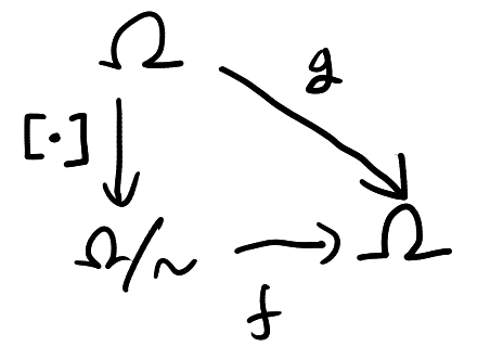
Definition
Let \(X\) be a \(n \times p\) matrix. We will define the singular value decomposition first in the case \(n \ge p\). The SVD consists of three matrix \(U \in \mathbb{R}^{n \times p}, \Sigma \in \mathbb{R}^{p \times p}\) and \(V \in \mathbb{R}^{p \times p}\) such that \(X = U\Sigma V^T\). The matrix \(\Sigma\) is required to be diagonal with non-negative diagonal entries \(\sigma_1 \ge \sigma_2 \ge \ldots \ge \sigma_p \ge 0\). These numbers are called the singular values of \(X\). The matrices \(U\) and \(V\) are required to orthogonal matrices so that \(U^TU=V^TV = I_p\), the \(p \times p\) identity matrix. Note that since \(V\) is square we also have \(VV^T=I_p\) however we won’t have \(UU^T = I_n\) unless \(n = p\).
In the case when \(n \le p\), we can define the SVD of \(X\) in terms of the SVD of \(X^T\). Let \(\widetilde{U} \in \mathbb{R}^{p \times n}, \widetilde{\Sigma} \in \mathbb{R}^{n \times n}\) and \(\widetilde{V} \in \mathbb{R}^{n \times n}\) be the SVD of \(X^T\) so that \(X^T=\widetilde{U}\widetilde{\Sigma}\widetilde{V}^T\). The SVD of \(X\) is then given by transposing both sides of this equation giving \(U = \widetilde{V}, \Sigma = \widetilde{\Sigma}^T=\widetilde{\Sigma}\) and \(V = \widetilde{U}\).
Construction
The SVD of a matrix can be found by iteratively solving an optimisation problem. We will first describe an iterative procedure that produces matrices \(U \in \mathbb{R}^{n \times p}, \Sigma \in \mathbb{R}^{p \times p}\) and \(V \in \mathbb{R}^{p \times p}\). We will then verify that \(U,\Sigma \) and \(V\) satisfy the defining properties of the SVD.
We will construct the matrices \(U\) and \(V\) one column at a time and we will construct the diagonal matrix \(\Sigma\) one entry at a time. To construct the first columns and entries, recall that the matrix \(X\) is really a linear function from \(\mathbb{R}^p\) to \(\mathbb{R}^n\) given by \(v \mapsto Xv\). We can thus define the operator norm of \(X\) via
\(\Vert X \Vert = \sup\left\{ \|Xv\|_2 : \|v\|_2 =1\right\},\)
where \(\|v\|_2\) represents the Euclidean norm of \(v \in \mathbb{R}^p\) and \(\|Xv\|_2\) is the Euclidean norm of \(Xv \in \mathbb{R}^n\). The set of vectors \(\{v \in \mathbb{R} : \|v\|_2 = 1 \}\) is a compact set and the function \(v \mapsto \|Xv\|_2\) is continuous. Thus, the supremum used to define \(\Vert X \Vert\) is achieved at some vector \(v_1 \in \mathbb{R}^p\). Define \(\sigma_1 = \|X v_1\|_2\). If \(\sigma_1 \neq 0\), then define \(u_1 = Xv_1/\sigma_1 \in \mathbb{R}^n\). If \(\sigma_1 = 0\), then define \(u_1\) to be an arbitrary vector in \(\mathbb{R}^n\) with \(\|u\|_2 = 1\). To summarise we have
\(v_1 \in \mathbb{R}^p\) with \(\|v_1\|_2 = 1\).
\(\sigma_1 = \|X\| = \|Xv_1\|_2\).
\(u_1 \in \mathbb{R}^n\) with \(\|u_1\|_2=1\) and \(Xv_1 = \sigma_1u_1\).
We have now started to fill in our SVD. The number \(\sigma_1 \ge 0\) is the first singular value of \(X\) and the vectors \(v_1\) and \(u_1\) will be the first columns of the matrices \(V\) and \(U\) respectively.
Now suppose that we have found the first \(k\) singular values \(\sigma_1,\ldots,\sigma_k\) and the first \(k\) columns of \(V\) and \(U\). If \(k = p\), then we are done. Otherwise we repeat a similar process.
Let \(v_1,\ldots,v_k\) and \(u_1,\ldots,u_k\) be the first \(k\) columns of \(V\) and \(U\). The vectors \(v_1,\ldots,v_k\) split \(\mathbb{R}^p\) into two subspaces. These subspaces are \(S_1 = \text{span}\{v_1,\ldots,v_k\}\) and \(S_2 = S_1^\perp\), the orthogonal compliment of \(S_1\). By restricting \(X\) to \(S_2\) we get a new linear map \(X_{|S_2} : S_2 \to \mathbb{R}^n\). Like before, the operator norm of \(X_{|S_2}\) is defined to be
The set \(\{v \in \mathbb{R}^p : \|v\|_2=1, v_j^Tv=0\text{ for } j=1,\ldots,k\}\) is a compact set and thus there exists a vector \(v_{k+1}\) such that \(\|Xv_{k+1}\|_2 = \|X_{|S_2}\|\). As before define \(\sigma_{k+1} = \|Xv_{k+1}\|_2\) and \(u_{k+1} = Xv_{k+1}/\sigma_{k+1}\) if \(\sigma_{k+1}\neq 0\). If \(\sigma_{k+1} = 0\), then define \(u_{k+1}\) to be any vector in \(\mathbb{R}^{n}\) that is orthogonal to \(u_1,u_2,\ldots,u_k\).
This process repeats until eventually \(k = p\) and we have produced matrices \(U \in \mathbb{R}^{n \times p}, \Sigma \in \mathbb{R}^{p \times p}\) and \(V \in \mathbb{R}^{p \times p}\). In the next section, we will argue that these three matrices satisfy the properties of the SVD.
Correctness
The defining properties of the SVD were given at the start of this post. We will see that most of the properties follow immediately from the construction but one of them requires a bit more analysis. Let \(U = [u_1,\ldots,u_p]\), \(\Sigma = \text{diag}(\sigma_1,\ldots,\sigma_p)\) and \(V= [v_1,\ldots,v_p]\) be the output from the above construction.
First note that by construction \(v_1,\ldots, v_p\) are orthogonal since we always had \(v_{k+1} \in \text{span}\{v_1,\ldots,v_k\}^\perp\). It follows that the matrix \(V\) is orthogonal and so \(V^TV=VV^T=I_p\).
The matrix \(\Sigma\) is diagonal by construction. Furthermore, we have that \(\sigma_{k+1} \le \sigma_k\) for every \(k\). This is because both \(\sigma_k\) and \(\sigma_{k+1}\) were defined as maximum value of \(\|Xv\|_2\) over different subsets of \(\mathbb{R}^p\). The subset for \(\sigma_k\) contained the subset for \(\sigma_{k+1}\) and thus \(\sigma_k \ge \sigma_{k+1}\).
We’ll next verify that \(X = U\Sigma V^T\). Since \(V\) is orthogonal, the vectors \(v_1,\ldots,v_p\) form an orthonormal basis for \(\mathbb{R}^p\). It thus suffices to check that \(Xv_k = U\Sigma V^Tv_k\) for \(k = 1,\ldots,p\). Again by the orthogonality of \(V\) we have that \(V^Tv_k = e_k\), the \(k^{th}\) standard basis vector. Thus,
Above, we used that \(\Sigma\) was a diagonal matrix and that \(u_k\) is the \(k^{th}\) column of \(U\). If \(\sigma_k \neq 0\), then \(\sigma_k u_k = Xv_k\) by definition. If \(\sigma_k =0\), then \(\|Xv_k\|_2=0\) and so \(Xv_k = 0 = \sigma_ku_k\) also. Thus, in either case, \(U\Sigma V^Tv_k = Xv_k\) and so \(U\Sigma V^T = X\).
The last property we need to verify is that \(U\) is orthogonal. Note that this isn’t obvious. At each stage of the process, we made sure that \(v_{k+1} \in \text{span}\{v_1,\ldots,v_k\}^\perp\). However, in the case that \(\sigma_{k+1} \neq 0\), we simply defined \(u_{k+1} = Xv_{k+1}/\sigma_{k+1}\). It is not clear why this would imply that \(u_{k+1}\) is orthogonal to \(u_1,\ldots,u_k\).
It turns out that a geometric argument is needed to show this. The idea is that if \(u_{k+1}\) was not orthogonal to \(u_j\) for some \(j \le k\), then \(v_j\) couldn’t have been the value that maximises \(\|Xv\|_2\).
Let \(u_{k}\) and \(u_j\) be two columns of \(U\) with \(j < k\) and \(\sigma_j,\sigma_k > 0\). We wish to show that \(u_j^Tu_k = 0\). To show this we will use the fact that \(v_j\) and \(v_k\) are orthonormal and perform “polar-interpolation“. That is, for \(\lambda \in [0,1]\), define
Rearranging and dividing by \(\sqrt{\lambda}\) gives,
\(2\sqrt{1-\lambda}\cdot \sigma_1\sigma_2 u_j^Tu_k \le \sqrt{\lambda}\cdot(\sigma_j^2-\sigma_k^2).\) for all \(\lambda \in (0,1]\)
Taking \(\lambda \searrow 0\) gives \(u_j^Tu_k \le 0\). Performing the same polar interpolation with \(v_\lambda’ = \sqrt{1-\lambda}v_j – \sqrt{\lambda}v_k\) shows that \(-u_j^Tu_k \le 0\) and hence \(u_j^Tu_k = 0\).
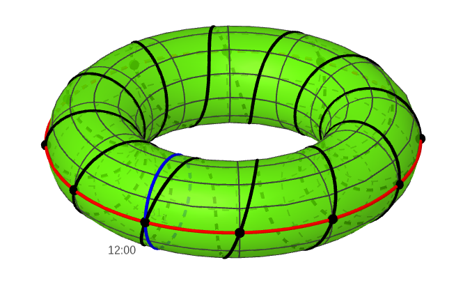
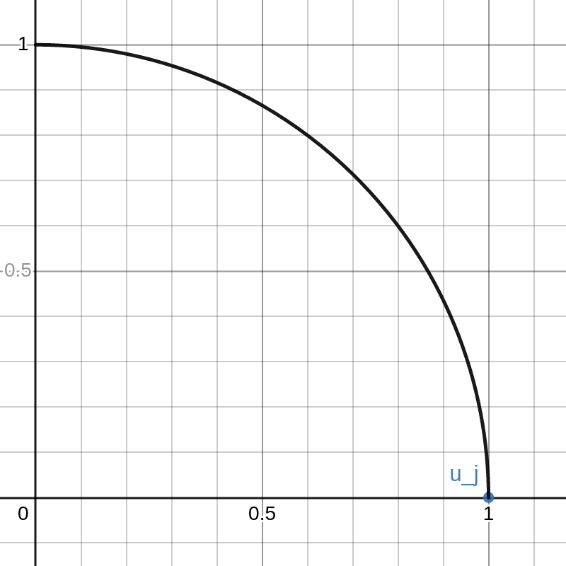
We have thus proved that \(U\) is orthogonal. This proof is pretty “slick” but it isn’t very illuminating. To better demonstrate the concept, I made an interactive Desmos graph that you can access here.
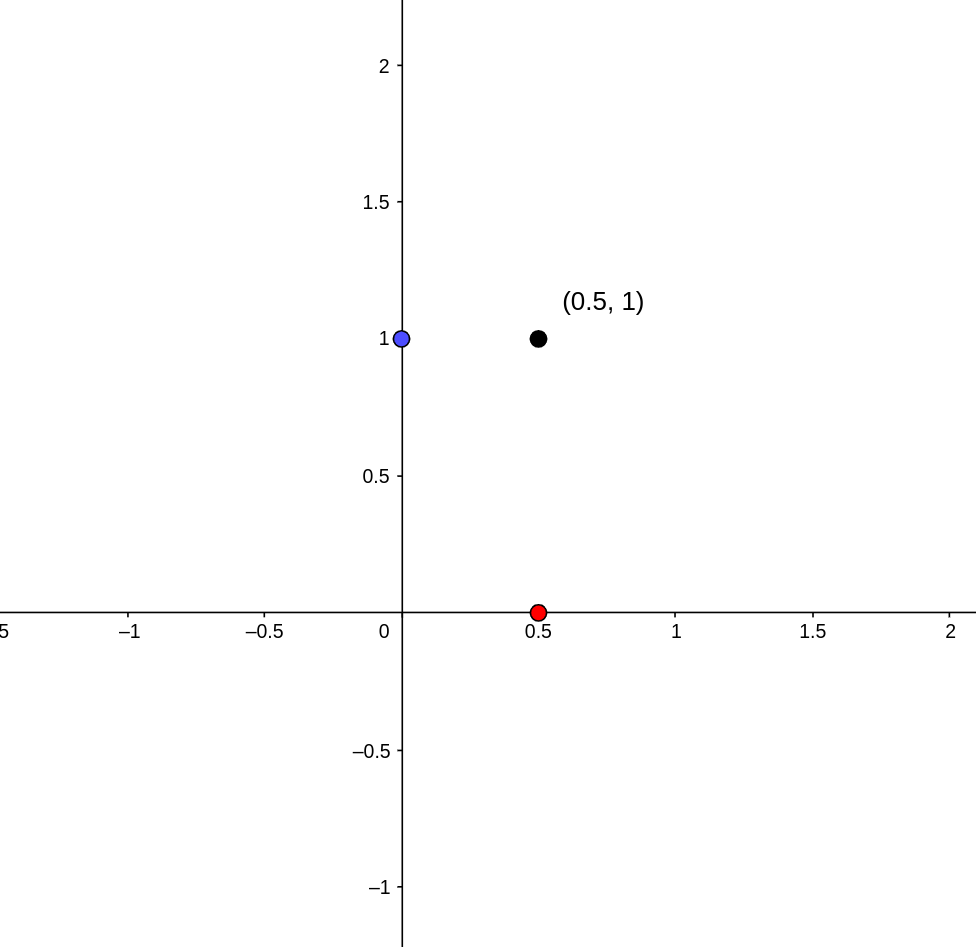
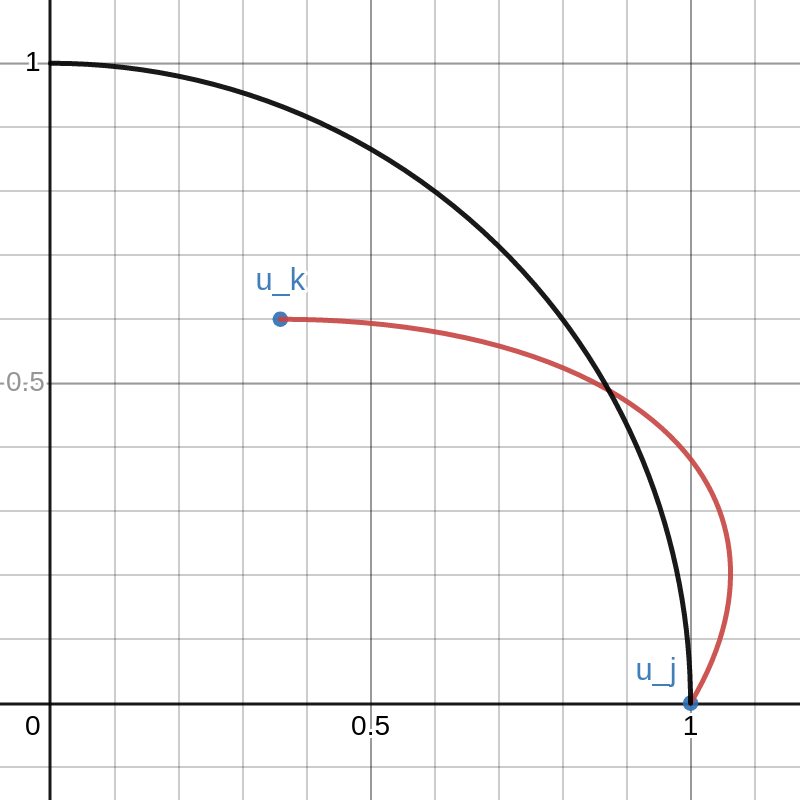
This graph shows example vectors \(u_j, u_k \in \mathbb{R}^2\). The vector \(u_j\) is fixed at \((1,0)\) and a quarter circle of radius \(1\) is drawn. Any vectors \(u\) that are outside this circle have \(\|u\|_2 > 1 = \|u_j\|_2\).
The vector \(u_k\) can be moved around inside this quarter circle. This can be done either cby licking and dragging on the point or changing that values of \(a\) and \(b\) on the left. The red curve is the path of
As \(\lambda\) goes from \(0\) to \(1\), the path travels from \(u_j\) to \(u_k\).
Note that there is a portion of the red curve near \(u_j\) that is outside the black circle. This corresponds to a small value of \(\lambda > 0\) that results in \(\|X v_\lambda\|_2 > \|Xv_j\|_2\) contradicting the definition of \(v_j\). By moving the point \(u_k\) around in the plot you can see that this always happens unless \(u_k\) lies exactly on the y-axis. That is, unless \(u_k\) is orthogonal to \(u_j\).