I used to have trouble understanding why inverting an \(n \times n\) matrix required the same order of operations as solving an \(n \times n\) system of linear equations. Specifically, if \(A\) is an \(n\times n\) invertible matrix and \(b\) is a length \(n\) vector, then computing \(A^{-1}\) and solving the equation \(Ax = b\) can both be done in \(O(n^3)\) floating point operations (flops). This surprised me because naively computing the columns of \(A^{-1}\) requires solving the \(n\) systems of equations
\(Ax = e_1, Ax=e_2,\ldots, Ax = e_n,\)
where \(e_1,e_2,\ldots, e_n\) are the standard basis vectors. I thought this would mean that calculating \(A^{-1}\) would require roughly \(n\) times as many flops as solving a single system of equations. It was only in a convex optimization lecture that I realized what was going on.
To solve a single system of equations \(Ax = b\), we first compute a factorization of \(A\) such as the LU factorization. Computing this factorization takes \(O(n^3)\) flops but once we have it, we can use it solve any new system with \(O(n^2)\) flops. Now to solve \(Ax=e_1,Ax=e_2,\ldots,Ax=e_n\), we can simply factor \(A\) once and the perform \(n\) solves using the factorization each of which requires an addition \(O(n^2)\) flops. The total flop count is then \(O(n^3)+nO(n^2)=O(n^3)\). Inverting the matrix requires the same order of flops as a single solve!
Of course, as John D Cook points out: you shouldn’t ever invert a matrix. Even if inverting and solving take the same order of flops, inverting is still more computational expensive and requires more memory.
I recently gave a talk on the Yang-Baxter equation. The focus of the talk was to state the connection between the Yang-Baxter equation and the braid relation. This connection comes from a system of interacting particles. In this post, I’ll go over part of my talk. You can access the full set of notes here.
Interacting particles
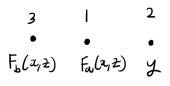
Imagine two particles on a line, each with a state that can be any element of a set \(\mathcal{X}\). Suppose that the only way particles can change their states is by interacting with each other. An interaction occurs when two particles pass by each other. We could define a function \(F : \mathcal{X} \times \mathcal{X} \to \mathcal{X} \times \mathcal{X}\) that describes how the states change after interaction. Specifically, if the first particle is in state \(x\) and the second particle is in state \(y\), then their states after interacting will be \(F(x,y) = (F_a(x,y), F_b(x,y))\) where \(F_a(x,y)\) is the new state of the first particle and \(F_b(x,y)\) is the state of the second particle.
Since the particles move past each other when they interact. Thus, to keep track of the whole system we need an element of \(\mathcal{X} \times \mathcal{X}\) to keep track of the states and a permutation \(\sigma \in S_2\) to keep track of the positions.
Three particles
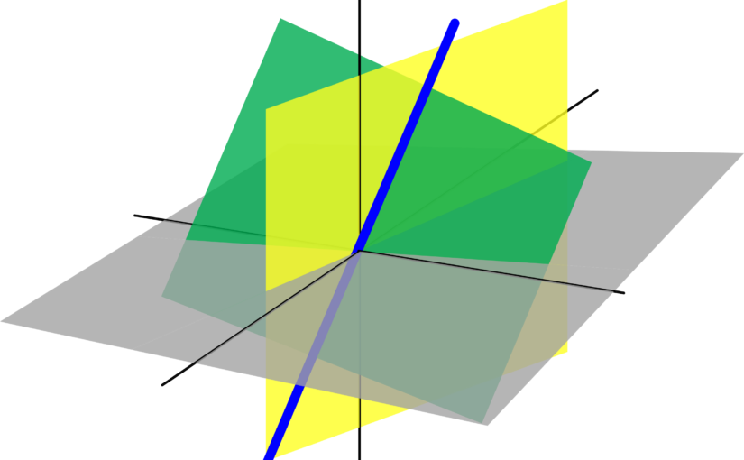
Now suppose that we have \(3\) particles labelled \(1,2,3\). As before, each particle has a state in \(\mathcal{X}\). We can thus keep track of the state of each particle with an element of \(\mathcal{X}^3\). The particles also have a position which is described by a permutation \(\sigma \in S_3\). The order the entries of \((x,y,z) \in \mathcal{X}^3\) corresponds to the labels of the particles not their positions. A possible configuration is shown below:
A possible configuration of the three particles. The above configuration is escribed as having states \((x,y,z) \in \mathcal{X}^3\) and positions \(132 \in S_3\).
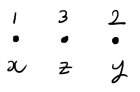
As before, the particles can interact with each other. However, we’ll now add the restriction that the particles can only interact two at a time and interacting particles must have adjacent positions. When two particles interact, they swap positions and their states change according to \(F\). The state and position of the remaining particle is unchanged. For example, in the above picture we could interact particles \(1\) and \(3\). This will produce the below configuration:
The new configuration after interacting particles \(1\) and \(3\) in the first diagram. The configuration is now described by the states \(F_{13}(x,y,z) \in \mathcal{X}^3\) and the permutation \(312 \in S_3\).
To keep track of how the states of the particles change over time we will introduce three functions from \(\mathcal{X}^3\) to \(\mathcal{X}^3\). These functions are \(F_{12},F_{13},F_{23}\). The function \(F_{ij}\) is given by applying \(F\) to the \(i,j\) coordinates of \((x,y,z)\) and acting by the identity on the remaining coordinate. In symbols,
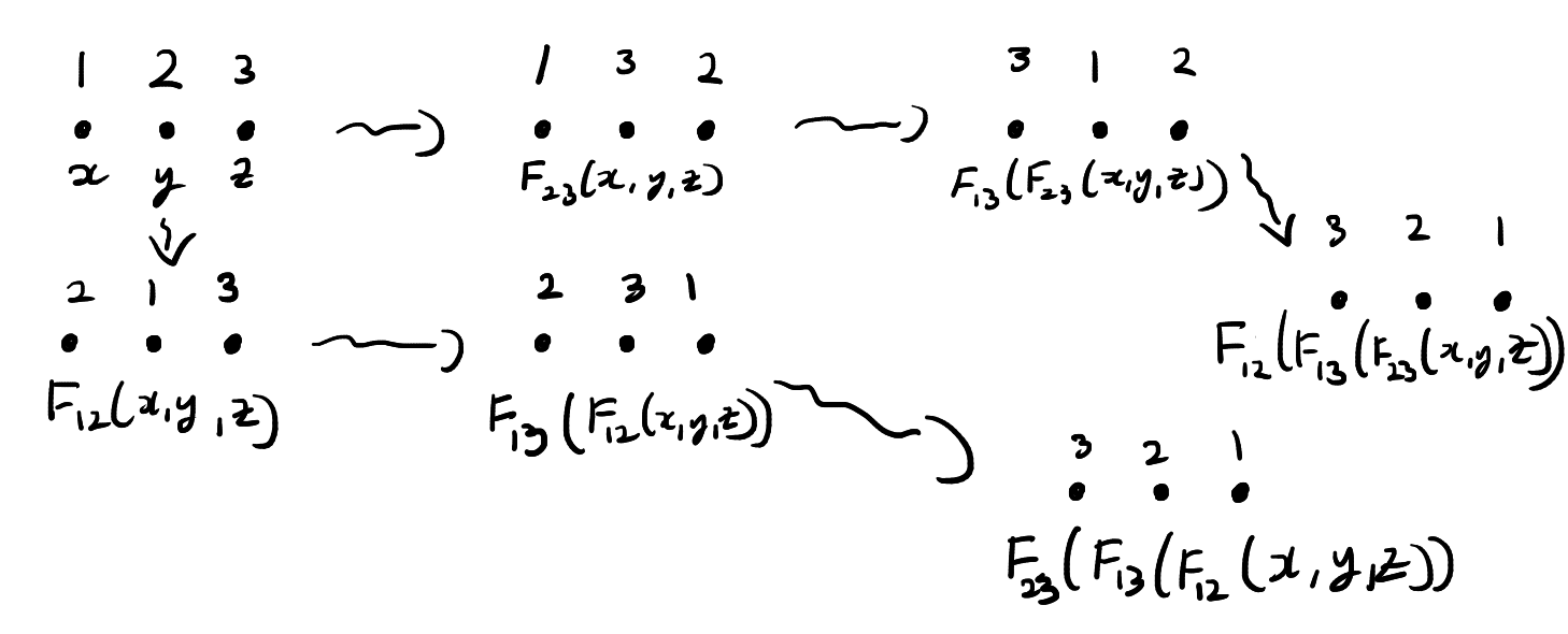
The function \(F_{ij}\) exactly describes how the states of the three particles change when particles \(i\) and \(j\) interact. Now suppose that three particles begin in position \(123\) and states \((x,y,z)\). We cannot directly interact particles \(1\) and \(3\) since they are not adjacent. We have to pass first pass one of the particles through particle \(2\). This means that there are two ways we can interact particles \(1\) and \(3\). These are illustrated below.
The two ways of passing through particle 2 to interact particles 2 and 3.
In the top chain of interactions, we first interact particles \(2\) and \(3\). In this chain of interactions, the states evolve as follows:
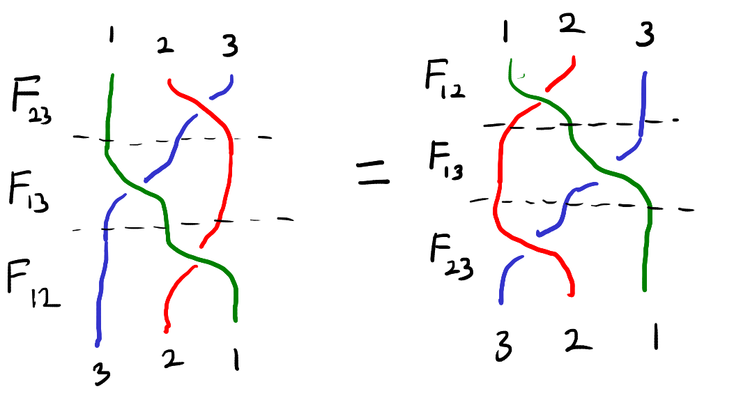
Note that after both of these chains of interactions the particles are in position \(321\). The function \(F\) is said to solve the Yang–Baxter equation if two chains of interactions also result in the same states.
Definition: A function \(F : \mathcal{X} \times \mathcal{X} \to \mathcal{X} \times \mathcal{X}\) is a solution to the set theoretic Yang–Baxter equation if,
This equation can be visualized as the “braid relation” shown below. Here the strings represent the three particles and interacting two particles corresponds to crossing one string over the other.
The braid relation.
Here are some examples of solutions to the set theoretic Yang-Baxter equation,
The identity on \(\mathcal{X} \times \mathcal{X}\).
The swap map, \((x,y) \mapsto (y,x)\).
If \(f,g : \mathcal{X} \to \mathcal{X}\) commute, then the function \((x,y) \to (f(x), g(y))\) is a solution the Yang-Baxter equation.
In the full set of notes I talk about a number of extensions and variations of the Yang-Baxter equation. These include having more than three particles, allowing for the particle states to be entangle and the parametric Yang-Baxter equation.
The \(p\)-norm of a vector \(x\in \mathbb{R}^n\) is defined to be:
\(\displaystyle{\Vert x \Vert_p = \left(\sum_{i=1}^n |x_i|^p\right)^{1/p}}.\)
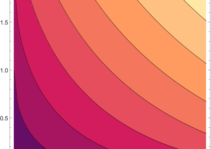
If \(p \ge 1\), then the \(p\)-norm is convex. When \(0<p<1\), this function is not convex and not actually a norm. In fact, the function \(x \mapsto \Vert x \Vert_p\) actually concave when \(0 < p < 1\) and all the entries of \(x\) are non-negative. This can be seen in the feature image for this post which shows that the contours of this function are concave for \(n = 2\).
On a recent exam for the course Convex Optimization, we were asked to prove this when \(p = 1/2\). In this special case, the mathematics simplifies nicely.
When \(p = 1/2\), the \(p\)-norm can be described as the squared sum of square roots. Specifically,
\(\displaystyle{\Vert x \Vert_{1/2} = \left(\sum_{i=1}^n \sqrt{|x_i|} \right)^2}.\)
Note that we can expand the square and rewrite the function as follows
\(\displaystyle{\Vert x \Vert_{1/2} = \sum_{i=1}^n\sum_{k=1}^n\sqrt{\left|x_i\right|} \sqrt{|x_k|} =\sum_{i=1}^n\sum_{k=1}^n \sqrt{|x_ix_k|}}.\)
If we restrict to \(x \in \mathbb{R}^n\) with \(x_i \ge 0\) for all \(i\), then this function simplifies to
\(\displaystyle{\Vert x \Vert_{1/2} =\sum_{i=1}^n\sum_{k=1}^n \sqrt{x_ix_k}},\)
which is a sum of geometric means. The geometric mean function \((u,v) \mapsto \sqrt{uv}\) is concave when \(u,v \ge 0\). This can be proved by calculating the Hessian of this function and verifying that it is negative semi-definite.
From this, we can conclude that each function \(x \mapsto \sqrt{x_ix_k}\) is also concave. This is because \(x \mapsto \sqrt{x_ix_k}\) is a linear function followed by a concave function. Finally, any sum of concave functions is also concave and thus \(\Vert x \Vert_{1/2}\) is concave.
Hellinger distance
A similar argument can be used to show that Hellinger distance is a convex function. Hellinger distance, \(d_H(\cdot,\cdot)\) is defined on pairs of probability distributions \(p\) and \(q\) on a common set \(\{1,\ldots,n\}\). For such a pair,
which certainly doesn’t look convex. However, we can expand the square and use the fact that \(p\) and \(q\) are probability distributions. This shows us that Helligener distance can be written as
Again, each function \((p,q) \mapsto \sqrt{p_iq_i}\) is concave and so the negative sum of such functions is convex. Thus, \(d_H(p,q)\) is convex.
The course
As a final comment, I’d just like to say how much I am enjoying the class. Prof. Stephen Boyd is a great lecturer and we’ve seen a wide variety of applications in the class. I’ve recently been reading a bit of John D Cook’s blog and agree with all he says about the course here.
where \(\sum_{i=1}^n \exp(a_i) > \sum_{j=1}^m \exp(b_j)\). Such expressions can be difficult to evaluate directly since the exponentials can easily cause overflow errors. In this post, I’ll talk about a clever way to avoid such errors.
If there were no terms in the second sum we could use the log-sum-exp trick. That is, to calculate
we can use the above method to separately calculate
\(\displaystyle{A = \log\left(\sum_{i=1}^n \exp(a_i) \right)}\) and \(\displaystyle{B = \log\left(\sum_{j=1}^m \exp(b_j)\right)}.\)
The final result we want is \(\log\left(\sum_{i=1}^n \exp(a_i) – \sum_{j=1}^m \exp(b_j) \right)\) which is equal to
\(\displaystyle{ \log(\exp(A) – \exp(B)) = A + \log(1-\exp(B-A))}.\)
Since \(A > B\), the right hand side of the above expression can be evaluated safely and we will have our final answer.
R code
The R code below defines a function that performs the above procedure
# Safely compute log(sum(exp(pos)) - sum(exp(neg)))
# The default value for neg is an empty vector.

logSumExp <- function(pos, neg = c()){
  max_pos <- max(pos)
  A <- max_pos + log(sum(exp(pos - max_pos)))

  # If neg is empty, the calculation is done
  if (length(neg) == 0){
    return(A)
  }

  # If neg is non-empty, calculate B.
  max_neg <- max(neg)
  B <- max_neg + log(sum(exp(neg - max_neg)))

  # Check that A is bigger than B
  if (A <= B) {
    stop("sum(exp(pos)) must be larger than sum(exp(neg))")
  }

  # log1p() is a built in function that accurately calculates log(1+x) for |x| << 1
  return(A + log1p(-exp(B - A)))
}
Evaluating this directly would quickly lead to errors since R (and most other programming languages) cannot compute \(200!\). However, R has the functions lfactorial() and lchoose() which can compute \(\log(i!)\) and \(\log\binom{n}{i}\) for large values of \(i\) and \(n\). We can thus put this expression in the general form at the start of this post
The beta-binomial model is a Bayesian model used to analyze rates. For a great derivation and explanation of this model, I highly recommend watching the second lecture from Richard McElreath’s course Statistical Rethinking. In this model, the data, \(X\), is assumed to be binomially distributed with a fixed number of trail \(N\) but an unknown rate \(\rho \in [0,1]\). The rate \(\rho\) is given a \(\text{Beta}(a,b)\) prior. That is the prior distribution of \(\rho\) has a density
The last expression is proportional to a beta density., specifically \(\rho | X \sim \text{Beta}(X+a, N-X+b)\).
The marginal distribution of \(X\)
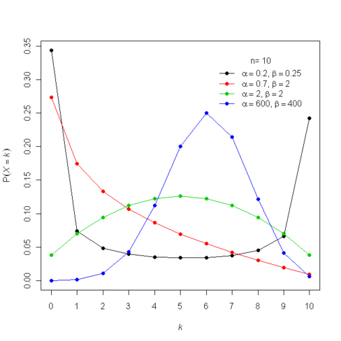
In the above model we are given the distribution of \(\rho\) and the conditional distribution of \(X|\rho\). To calculate the distribution of \(X\), we thus need to marginalize over \(\rho\). Specifically,
This distribution is called the beta-binomial distribution. Below is an image from Wikipedia showing a graph of \(p(X)\) for \(N=10\) and a number of different values of \(a\) and \(b\). You can see that, especially for small value of \(a\) and \(b\) the distribution is a lot more spread out than the binomial distribution. This is because there is randomness coming from both \(\rho\) and the binomial conditional distribution.