Logistic regression is a technique for analyzing data where the dependent variable is binary. In this post, we will introduce logistic regression and then discuss how to fit a logistic regression model using only aggregated count data.
Logistic regression overview
Logistic regression can be used when the dependent variable \(Y_i\) is binary. For example, in a medical study the dependent variable might be whether or not a patient developed a disease. In this case \(Y_i=1\) will mean that patient \(i\) did develop the disease and \(Y_i=0\) will mean that that patient \(i\) did not develop the disease. In logistic regression, the independent variables can either be categorical or quantitative. In the medical example, the type of treatment received could be a categorical independent variable and the age of the patient could be a quantitative independent variable.
Logistic regression models the probability that \(Y_i=1\) given the independent variables. If \(X_{i,1},\ldots,X_{p,1}\) are the values of the independent variables for patient \(i\), then logistic regression assumes that
\(\mathrm{Pr}(Y_i=1) = \sigma(\beta_0 + \beta_1 X_{i,1} + \cdots +\beta_p X_{i,p}) \),
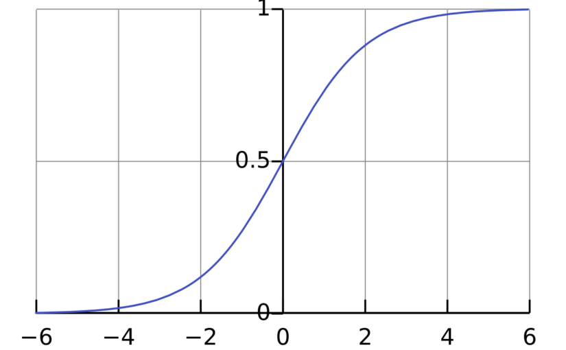
where \(\mathrm{Pr}(Y_i=1)\) is the probability that \(Y_i = 1\), \(\sigma\) is the logistic function \(\sigma(x) = \frac{1}{1+\exp(-x)}\) and \(\beta_0,\beta_1,\ldots,\beta_p\) are parameters that will be estimated from the data. The interpretation of the parameter \(\beta_j\) is that if \(X_{i,j}\) increases by 1 unit and all the other independent variables are fixed, then the odds \(\frac{\mathrm{Pr}(Y_i=1)}{\mathrm{Pr}(Y_i=0)}\) will increase by a factor of \(\exp(\beta_j)\).
Logistic regression models can be fit to data in using the function glm() in the programming language R. For example, to fit a logistic regression model with dependent variable disease and independent variables treatment and age, you can use the code
logistic_model <- glm(
          disease ~ treatment + age,
          data = data,
          family = binomial)
To view the estimates of the parameters of the model (as well as standard errors and p-values), you can run the code summary(logistic_model).
Logistic regression with aggregate data
If all of the independent variables are categorical, then it is possible to fit a logistic model with the aggregate count data. For example, the table below is from a study from the 1980s/1990s on the effect of AZT treatment on slowing the development of AIDS.1
| Race | AZT use | Symptoms | No Symptoms |
| Black | Yes | 11 | 52 |
| Black | No | 12 | 43 |
| White | Yes | 14 | 93 |
| White | No | 32 | 81 |
The study featured 338 veterans who were positive for HIV and were beginning to show signs of faltering immune systems. The veterans were randomly assigned to either immediately receive AZT or to receive AZT once their T-cells showed signs of severe immune weakness. The table records whether the veterans received AZT immediately, the race of the veterans and whether they developed AIDS in the three year study period.
The table above shows aggregated data. The table reports the number of people for each combination of treatment, race and disease status. The table does not report individual patient data. However, it is it possible to fit a logistic regression model to the aggregate data.2 We just need to make some small changes to the R code.
To describe the changes, let’s first review what we would do with the patient level data. Suppose we had a dataset individual_data that had a row for each veteran and had columns race, azt_use and developed_symptoms that record the veteran’s race, AZT use and whether they developed symptoms. Our goal is to fit a logistic regression model where dependent variable \(Y_i\) is a binary variable with \(Y_i=1\) meaning that the patient did develop symptoms. The independent variables are race and AZT use. With the individual data, we could use the following:
individual_model <- glm(
    developed_symptoms ~ race + azt_use,
    family = binomial,
    data = individual_data)
Now suppose that we only have the aggregate data in a table called aggregate_data. This table has columns race, azt_use, symptoms and no_symptoms like the table presented above. To fit the logistic model with this data, there are two options.
- The first option is to replace the independent variable
developed_symptomsin the individual model withcbind(symptoms, no_symptoms). The functioncbindcreates a matrix with two columns recording the number of people with and without symptoms for each combination of race and AZT use. We also need to tell R to use the aggregate data. Here is the R code:
aggregate_model_1 <- glm(
    cbind(symptoms, no_symptoms) ~ race + azt_use,
    family = binomial,
data = aggregate_data- The other option is to replace the independent variable
developed_symptomswith the proportion of people who developed symptoms. To use this option, it is also necessary to compute the total number of people for each combination of race and AZT use. These totals are used as weights in the logistic regression. In the code below, we first compute the proportion and the total number of people and then fit the model.
aggregate_data$total <- aggregate_data$symptoms + aggregate_data$no_symptomsaggregate_data$proportion <- aggregate_data$symptoms / aggregate_data$total
aggregate_model_2 <- glm(
proportion ~ race + azt_use,
family = binomial, data = aggregate_data)Results
Both aggregate_model_1 and aggregate_model_2 produce the exact same parameter estimates, standard errors and p-values. More importantly, if we had the individual data, individual_model would also have the same results. We can actually check this by “de-aggregating” the data. This involves making a dataset with, for example, 11 rows with race = "Black", azt_use = "Yes" and developed_symptoms = 1 so that these 11 rows represent the 11 veterans in the first category of the table above.
All three logisitic regression models give the same final results:
| Estimate | Standard error | p-value | |
| Intercept | -1.07 | 0.263 | 4e-05 |
| raceWhite | 0.05 | 0.289 | 0.848 |
| atz_useYes | -0.719 | 0.279 | 0.01 |
The parameter estimates shows that Black and White veterans had approximately the same chance of developing symptoms (assuming that they either both received ATZ treatment or that neither of them received ATZ treatment). On the other hand, the parameter estimate for ATZ use is significant. The estimated value of -0.719 can be interpreted as follows. If the race of the veteran is held constant, then the odds of developing symptoms was half as high for the veterans who immediately took ATZ than for those who waited. In mathematical symbols:
\(\frac{\mathrm{Pr}(\text{developed symptoms} \mid \text{ATZ immediately})}{\mathrm{Pr}(\text{did not develop symptoms} \mid \text{ATZ immediately})}\)
is roughly equal to
\( 0.5 \times \frac{\mathrm{Pr}(\text{developed symptoms} \mid \text{waited for ATZ use})}{\mathrm{Pr}(\text{did not develop symptoms} \mid \text{waited for ATZ})} \)
The specific value of 0.5 comes from the fact that \(\exp(-0.719) \approx 0.5\). Section 5.4.2 of Categorical Data Analysis by Alan Agresti discusses the interpretation of the parameter estimates for this example in more detail.
R code for fitting all three models is available at the end of this post.3
Footnotes
- The data on AZT is from Table 5.6 of Alan Agresti’s Categorical Data Analysis (3rd edition) https://onlinelibrary.wiley.com/doi/book/10.1002/0471249688, https://mybiostats.wordpress.com/wp-content/uploads/2015/03/3rd-ed-alan_agresti_categorical_data_analysis.pdf ↩︎
- In statistical jargon, the aggregate data are sufficient statistics for the logistic regression model. ↩︎
- R code: ↩︎
# Aggregate data from Agresti Table 5.6
aggregate_data <- data.frame(
  race = c("Black", "Black", "White", "White"),
  atz_use = c("yes", "no", "yes", "no"),
  symptoms = c(11, 12, 14, 32),
  no_symptoms = c(52, 43, 93, 81)
)

# Aggregate model 1 using cbind()
aggregate_model_1 <- glm(
  cbind(symptoms, no_symptoms) ~ race + atz_use,
  data = aggregate_data,
  family = binomial)

# Aggregate model 2 using proportions and weights
aggregate_data$total <- aggregate_data$symptoms + aggregate_data$no_symptoms
aggregate_data$proportion <- aggregate_data$symptoms / aggregate_data$total

aggregate_model_2 <- glm(
  proportion ~ race + atz_use,
  data = aggregate_data,
  weights = total,
  family = binomial)

# Individual model

# Function to "de-aggregate"
deaggregate_data <- function(aggregate_data) {
  # Create an empty list to store rows
  rows_list <- list()

  # Iterate through each row of aggregate data
  for (i in 1:nrow(aggregate_data)) {
    race_val <- aggregate_data$race[i]
    atz_val <- aggregate_data$atz_use[i]
    n_symptoms <- aggregate_data$symptoms[i]
    n_no_symptoms <- aggregate_data$no_symptoms[i]

    # Create rows for those with symptoms
    if (n_symptoms > 0) {
      rows_list[[length(rows_list) + 1]] <- data.frame(
        race = rep(race_val, n_symptoms),
        atz_use = rep(atz_val, n_symptoms),
        developed_symptoms = rep(1, n_symptoms)
      )
    }

    # Create rows for those without symptoms
    if (n_no_symptoms > 0) {
      rows_list[[length(rows_list) + 1]] <- data.frame(
        race = rep(race_val, n_no_symptoms),
        atz_use = rep(atz_val, n_no_symptoms),
        developed_symptoms = rep(0, n_no_symptoms)
      )
    }
  }

  # Combine all rows into one data frame
  do.call(rbind, rows_list)
}

individual_data <- deaggregate_data(aggregate_data)

individual_model <- glm(
  developed_symptoms ~ race + atz_use,
  data = individual_data,
  family = binomial
)

# Compare models
summary(aggregate_model_1)
summary(aggregate_model_2)
summary(individual_model)


